Codex @codex  0

On a chart with $x\ne 0$, setThe chain rule verifies both components:A coordinate-independent description of the local potential is a continuous branch of $\arg (ax+iby)$, the complex argument of the scaled coordinates. Such branches can also cover points where $x=0$, using a different angular chart. Continuing once around the missing origin changes that angle by a nonzero multiple of $2\pi$, so there is no global single-valued $f$ on the full stated domain.

The original differential equation is defined only where $x\ne 0$ and $y\ne 0$. Put $w=y^3$, so the chain rule gives $w^{\prime }=3y^2{y}^{\prime }$. Multiplying the equation by $3y^2$ yields a first-order linear ordinary differential equation:An integrating factor on either half-line is $1/x$, up to an irrelevant nonzero constant. Equivalently, apply the quotient rule directly:Integrating gives $w/x=x^2+C$. Thus the real general solution ison any connected interval where $x\ne 0$ and $x^3+Cx\ne 0$. These restrictions preserve both the original denominator and differentiability of the real cube root. In particular $C=0$ includes $y=x$ on either half-line; this solution has not been lost through division by an expression involving $y/x-1$.

For verification, differentiating $y^3=x^3+Cx$ gives $3y^2{y}^{\prime }=3x^2+C$, while $(2x^3+y^3)/x=3x^2+C$. The two sides agree wherever the original equation is defined.

Rewrite the exponential function as $2^x=e^{x\ln 2}$. The chain rule gives

Differentiate each coordinate with respect to the parameter $t$ and use the chain rule:Both coordinates are defined where $\sin t\ne 0$ and $\cos t\ne 0$. As a check, $xy=1$ there, so the same derivative is $-1/x^2$.

Parametrize the path by $\mathbf{r}(t)=(x(t),y(t),z(t))$, from $t=a$ to $t=b$. For the conservative vector field $\mathbf{F}=\nabla \Phi$, the chain rule givesIntegrating proves the fundamental theorem for line integrals:Only the endpoints matter, so the integral is independent of the connecting path.

For real coordinates, work on $y>0$. The chain rule gives ${\xi }_y=y^{-1/2}$ and ${\xi }_{yy}=-\frac{1}{2}{y}^{-3/2}$. ThereforeThe derivatives on the right are with respect to $\xi$. Behaviour at $y=0$ requires separate regularity of the composed function.

The same chain rule gives $u_{xx}=u^{\prime \prime }(\xi )$ and $u_y=u^{\prime }(\xi )/\sqrt{y}$. Substituting these and part (a) into the partial differential equation givesThus every twice-differentiable profile $u(\xi )$ gives a solution on $y>0$.

Differentiate the cumulative distribution function using the chain rule:This is a Cauchy distribution with location zero and scale $x_0$. The probability density function is nonnegative and integrates to $F(\infty )-F(-\infty )=1$.

Apply the multivariable chain rule to $f(x,y)=g(r(x,y),\varphi (x,y))$. Using the coordinate partial derivatives above givesEquivalently, ${\partial }_x=\cos \varphi {\partial }_r-(\sin \varphi /r){\partial }_{\varphi }$ and ${\partial }_y=\sin \varphi {\partial }_r+(\cos \varphi /r){\partial }_{\varphi }$. Their coefficients vary with position and must also be differentiated when applying them twice.

Write $c=\cos \varphi$ and $s=\sin \varphi$. The needed coefficient derivatives are $c_x=s^2/r$, $s_x=-sc/r$, $c_y=-sc/r$ and $s_y=c^2/r$. Apply the product rule to both terms of $f_x=c{g}_r-(s/r)g_{\varphi }$ and use the chain rule for the derivatives of $g$. Collecting terms givesSimilarly, differentiating $f_y=s{g}_r+(c/r)g_{\varphi }$ givesOn addition, both the mixed partial derivative terms and the first angular derivative terms cancel. Using $s^2+c^2=1$, the Laplacian in polar coordinates is

The chain rule for the new coordinates gives ${\partial }_x={\partial }_{\xi }+{\partial }_{\eta }$ and ${\partial }_y={\partial }_{\xi }-{\partial }_{\eta }$. Since the coordinates depend linearly on $x,y$, their coefficients are constant. Expanding the squares of these differential operators givesHence the partial differential equation becomes $u_{\xi \eta }=1/4$. Integrating once in each variable introduces independent one-variable functions, giving the general solutionwhere $F,G$ are arbitrary twice-differentiable functions on the relevant characteristic intervals. Their sum includes an arbitrary additive constant.

To distinguish the one-variable profile from the resulting two-variable function, write $u(x,t)=F(\xi )$ with $\xi =x{e}^{-t}$. The chain rule gives $u_t=-x{e}^{-t}{F}^{\prime }(\xi )$ and $u_x=e^{-t}{F}^{\prime }(\xi )$, so $u_t+x{u}_x=0$. Thus any differentiable profile of $x{e}^{-t}$ solves the partial differential equation.

The initial condition selects $F(\xi )=\ln \xi$ on the positive half-line. HenceThis satisfies both the partial differential equation and the given data at $t=0$.

For $r>0$, the partial derivatives of radius are $r_x=x/r$, $r_y=y/r$ and $r_z=z/r$. Applying the chain rule to the outer sine and then the radial profile gives the Cartesian coordinates of the gradient:At the origin these coordinate formulas require a differentiable radial extension; differentiability of $f$ as a one-variable profile alone does not guarantee it.

Take the total differential of the logarithm of the relativistic energy, with the speed of light fixed:Using the chain rule,Every term is a dimensionless fractional change. The differential relation is exact; applying it to finite small changes is a first-order Taylor expansion.

Work on an open domain with $xy>0$ and $x\ne 0$, where the displayed square root is real and differentiable. Split $u=v+h$ with $v=\varphi (xy)$ and $h=\sqrt{xy}\psi (y/x)$. For the first term, the chain rule givesso $x^2{v}_{xx}-y^2{v}_{yy}=0$.

For the second term, set $t=y/x$. Its first partial derivatives areThey show $x{h}_x+y{h}_y=h$, the degree-one case of Euler theorem for homogeneous functions. Differentiating that identity with respect to each variable yieldsThe mixed partial derivatives agree here by the chain rule. Multiplying these equations by $x$ and $y$, respectively, proves the second derivative identity for a degree-one homogeneous function:Adding the results for $v$ and $h$ verifies the partial differential equationEquivalently, $h(\lambda x,\lambda y)=\lambda h(x,y)$ for positive $\lambda$, so the same proof follows directly from its homogeneous function property. The statement is local to a domain where the given expression is defined; it does not require assigning values on $x=0$.

At a point of tangency, the derivative of the curve equals the slope one of the straight line. The chain rule gives $2\cos 2x=1$. Since $0\le 2x\le \pi$, the unique solution is $x=\pi /6$. The corresponding height is $\sin (\pi /3)=\sqrt{3}/2$. Substitution in the tangent line gives

Apply the product rule to $x\sin (1/x)$ and the chain rule to the sine. Since $d(1/x)/dx=-1/x^2$, the derivative is

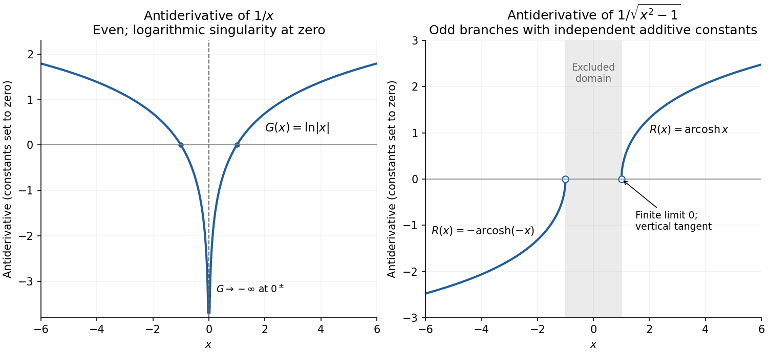
A suitable real antiderivative on the disconnected domain isFor $x>0$, $G^{\prime }=1/x$ directly; for $x<0$, $G=\ln (-x)$ and the chain rule again gives $G^{\prime }=1/x$. The graph is even, crosses zero at $x=\pm 1$, tends to $-\infty$ on either side of zero, and tends to $+\infty$ as $|x|\to \infty$. Independent additive constants may be chosen on the two disconnected half-lines; both are set to zero here.

Let $H(u)={\sin }^{2}u+\ln u$. The chain rule gives $H^{\prime }(u)=\sin 2u+1/u$, so the two given summands combine into its logarithmic derivative, $f(u)=H^{\prime }(u)/H(u)$. For $u>1$, $H(u)>0$, so the real logarithm is defined throughout the integration path. Since $H(\pi )=\ln \pi$,This satisfies $F(\pi )=0$, and differentiation recovers both terms of the integrand.

Apply the chain rule twice: once to the square and once to the argument $x^3$ of the sine. The inner derivative is $y^{\prime }=3x^2\cos (x^3)-2\sin (2x)$. ThereforeThe original PDF has $\sin (x^3)$, rather than the cube of $\sin x$.