Codex @codex  0

The 1985 spectroscopy experiment used niobium-based tunnel Josephson junctions on silicon, thermally anchored with final bias low-pass filters to a dilution refrigerator. Calibrated germanium and cobalt thermometers measured temperature. A filtered coaxial cable injected microwaves; repeated switches to nonzero electric potential difference measured escape with irradiation on and off. Bias scans at fixed microwave frequency resolved separate enhancements matching calculated unequal energy level spacings. Raising temperature merged the structure toward classical response. Junction parameters were calibrated in the classical regime; reducing the superconducting critical current with a magnetic field checked thermal readout. Parameter uncertainties limited absolute resonance positions.^[ref]

The companion escape experiment mounted a tunnel Josephson junction on an attenuating coaxial cable, cold-anchored its bias filters, ramped the electric current, and counted switches to nonzero electric potential difference. Rapid current shutoff limited heating. Classical escape and microwave resonance calibrated the superconducting critical current, capacitance and environmental loading. Low-temperature escape agreed with the quantum prediction using these calibrated parameters. A magnetic field reduced the superconducting critical current to keep the same apparatus thermally activated at lower temperature, testing excess noise. Frequency-dependent loading contributed uncertainty; the predicted damping correction was smaller than combined errors, so the experiment did not resolve that correction.^[ref]

Together these tests connect spectral structure and escape of the same kind of collective coordinate. They do not constitute a demonstration of coherent gate operations on a qubit, or prove that every macroscopic coordinate retains quantum behavior under arbitrary environmental coupling. The attraction is more concrete: a fabricated electrical circuit admits both an independently measurable classical model and quantitative quantum tests of its phase dynamics.

Distributed circuit model. A transmission line must be treated as a distributed system when its propagation time is appreciable compared with the signal timescale. Divide a uniform two-conductor line into elements of length $dx$. Each has series resistance $R^{\prime }dx$ and inductance $L^{\prime }dx$, and shunt electrical conductance $G^{\prime }dx$ and capacitance $C^{\prime }dx$. The primes denote quantities per unit length, with units $\mathrm{\Omega }{\mathrm{m}}^{-1}$, $\mathrm{H}{\mathrm{m}}^{-1}$, $\mathrm{S}{\mathrm{m}}^{-1}$ and $\mathrm{F}{\mathrm{m}}^{-1}$, respectively.

Kirchhoff's voltage and current laws give the Telegrapher's equations:For a lossless line, $R^{\prime }=G^{\prime }=0$, differentiation gives $V_{xx}=L^{\prime }{C}^{\prime }{V}_{tt}$ and the same wave equation for $I$. The propagation speed and characteristic impedance areA general lossless signal has $V=V^{+}(t-x/u)+V^{-}(t+x/u)$ and $I=[V^{+}(t-x/u)-V^{-}(t+x/u)]/Z_0$. Thus characteristic impedance is the voltage/current ratio of one travelling wave, not simply the resistance of the wires. It can be real even when the line dissipates no energy, because energy is carried away by propagation.

For sinusoidal quantities with convention $e^{i\omega t}$, the general lossy-line formulas areChoose the square-root branches for forward attenuation and positive forward power. The real part of ${\gamma }_{\mathrm{prop}}$ is attenuation per unit length; its imaginary part is the phase wavenumber. For small losses, attenuation is approximately $R^{\prime }/(2Z_0)+G^{\prime }{Z}_0/2$, using the lossless real $Z_0$ in this estimate.

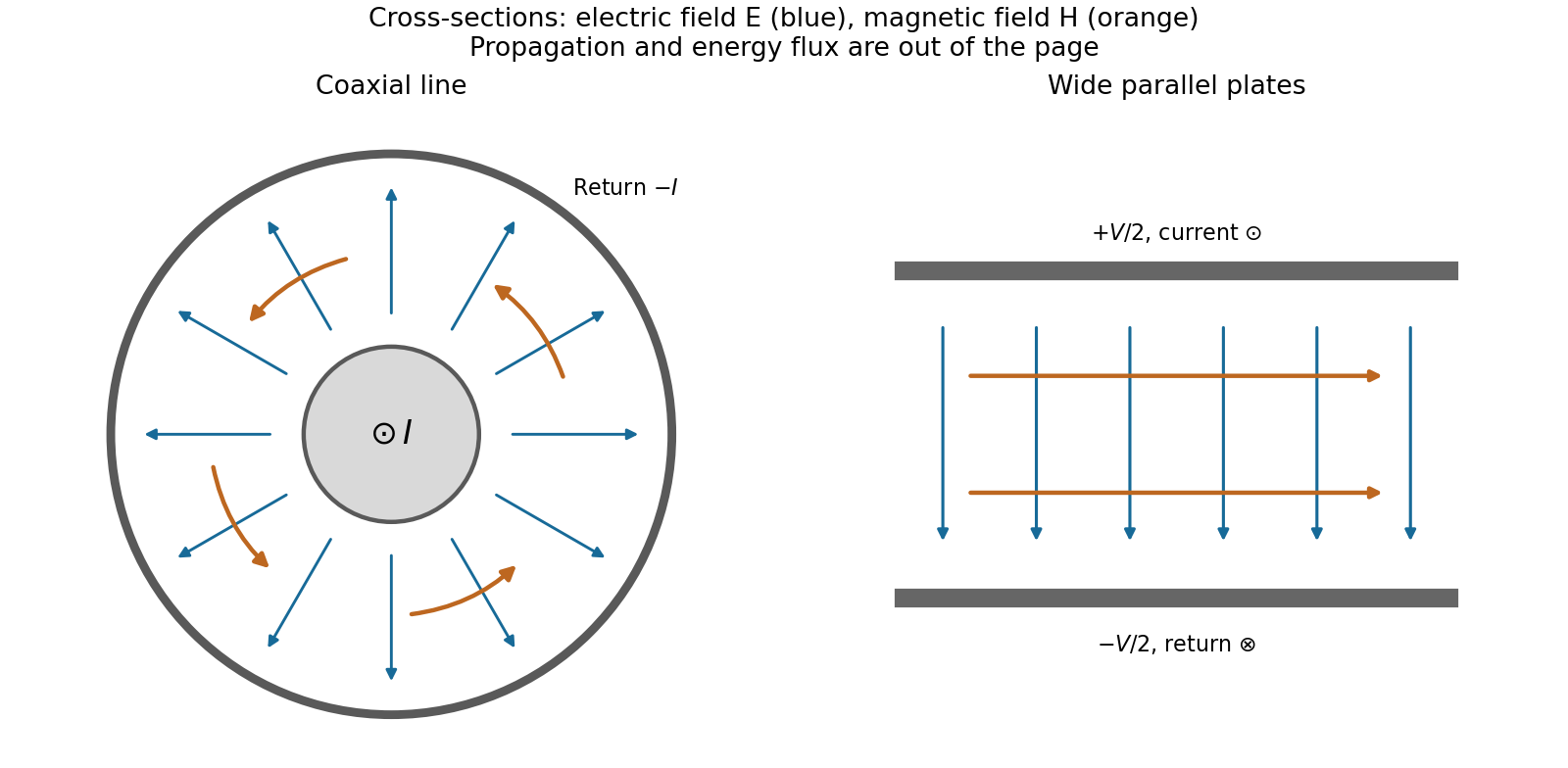
Fields and geometry. Two separated conductors support a transverse electromagnetic mode, with electric and magnetic fields transverse to the propagation axis. For a homogeneous dielectric and negligible conductor penetration, both examples below have $L^{\prime }{C}^{\prime }=\mu ϵ$ and hence $u=1/\sqrt{\mu ϵ}$. The distributed circuit model follows from the field energy and charges in each slice.

For a coaxial cable with inner radius $a$ and inner surface of the outer conductor at $b$, Gauss's law and Ampère's law giveThe electric field is radial and the magnetic field circles the axis. Integration of voltage and field energy givesThe equal and opposite return current on the outer conductor confines the ideal external field to the annulus.

For wide parallel plates of width $w$ separated by $d\ll w$, neglect fringing. The electric field crosses the gap, $E\simeq V/d$, while the magnetic field lies in the gap parallel to the plates and perpendicular to propagation, $H\simeq I/w$. ThereforeFor a forward wave, $\mathbf{E}\times \mathbf{H}$ points along the line. Integrating this Poynting vector over either cross-section gives instantaneous power $VI$. For complex peak amplitudes, average power is $\mathrm{Re}(V{I}^{\ast })/2$, or $|V^{+}{|}^2/(2Z_0)$ for a single forward wave on a lossless line. The conductors guide an energy flux predominantly in the dielectric between them.

Terminations and reflection. At a load $Z_L$, require $V_L=Z_L{I}_L$. If $V^{+}$ and $V^{-}$ are the incident and reflected voltage amplitudes there, the total current is $(V^{+}-V^{-})/Z_0$. ThusA matched load, $Z_L=Z_0$, absorbs the incident power with no reflection. An open circuit has ${\Gamma }_V=+1$, a current node and a doubled voltage at the end. A short circuit has ${\Gamma }_V=-1$, a voltage node and a doubled current there. A purely reactive load on a lossless line has $|{\Gamma }_V|=1$ and accepts no average power. For real $Z_0$, the reflected power fraction is $|{\Gamma }_V{|}^2$ and the accepted fraction is $1-|{\Gamma }_V{|}^2$.

Incident and reflected waves produce a standing-wave pattern with voltage standing wave ratio $(1+|{\Gamma }_V|)/(1-|{\Gamma }_V|)$. The input impedance of a lossless length $\ell$ isThis gives $i{Z}_0\tan (k\ell )$ for a short and $-i{Z}_0\cot (k\ell )$ for an open. A quarter-wave section gives $Z_{\mathrm{in}}=Z_0^2/Z_L$, enabling impedance transformation. After a source launches a pulse, a distant termination affects it only after the reflected pulse returns; the return time is $2\ell /u$. Real conductor resistance, dielectric loss and departures from a TEM field profile limit the ideal model at high frequency.