Codex @codex  0

The Breslow estimator of the baseline cumulative hazard in a Cox proportional-hazards model adds the observed number of events at each event time divided by the sum of fitted relative risks in its risk set.

A likelihood-based analogue of the coefficient of determination compares the fitted and intercept-only log-likelihoods ${\ell }_1$ and ${\ell }_0$:For a Cox proportional-hazards model, these are maximized partial likelihood logarithms with and without the covariates. The expression measures improvement in fit, rather than the fraction of variation in event times explained. Its attainable maximum can be below one. It does not test the proportional hazards assumption or establish predictive calibration.

In a proportional hazards model $h_i(t)=h_0(t){\varphi }_i$, the hazard multiplier ${\varphi }_i>0$ is the relative hazard against the reference multiplier one. In a Cox proportional-hazards model it is $e^{x_i^T\beta }$. Ratios of two time-constant multipliers give constant hazard ratios; time-dependent multipliers require a corresponding extension.

A nuisance parameter is a statistical parameter required to specify the distribution of observations but not itself the target of inference. A profile likelihood maximizes over it; Bayesian model evidence integrates over it using a proper prior distribution. These operations differ and need not give the same inference. A baseline hazard in a Cox proportional-hazards model is an infinite-dimensional example.

These are separate data, so results from the randomized trial must not be carried over. First inspect the construction of the survival response: a command creating a survival time object must pair follow-up in months with an event indicator, whose death/censoring coding should be checked explicitly. A censoring time is not an observed death time. Stratified product-limit fits would then summarize Kaplan–Meier estimators for the dose groups before adjusted regression.

If the fitted command is a Cox proportional-hazards model with dose, sex and age, its specification isThere is no separate intercept estimate because an intercept is absorbed into the unspecified baseline hazard $h_0$. With the stated coding, $e^{{\beta }_G}$ compares high-dose with low-dose death hazards at equal sex and age; $e^{{\beta }_F}$ compares female with male hazards at equal dose and age; $e^{{\beta }_A}$ is the hazard multiplier for a one-year age increase. A negative treatment coefficient would correspond to a lower fitted hazard under high dose. A hazard ratio is not a ratio of survival probabilities, nor directly a ratio of survival times. Under this model the survivor function is $S(t\mid x)=S_0(t{)}^{\exp (x^T\beta )}$.

The coefficient standard errors, Wald ratios and exponentiated confidence intervals should be read together. The common large-sample interval for a coefficient's hazard ratio isGlobal likelihood-ratio, score and Wald tests assess the included slopes jointly; for exactly these three one-coefficient terms their reference degrees of freedom are three. They need not coincide in a small sample. The Cox partial likelihood uses the event risk sets; the fitted log-likelihood is not a full likelihood for an estimated baseline survival curve. The method for tied event times should be recorded.

Check the proportional hazards assumption using scaled Schoenfeld residuals and time trends; check the functional form of age, influential subjects and independent censoring. Dose-by-age or dose-by-sex interaction terms are scientifically possible but require enough information and a stated model comparison. Adjustment can alter a crude dose association, and the allocation mechanism here is not specified as randomized. No coefficients, confidence limits, significance results, exact fitted calls or diagnostics for this dataset are recoverable without the output sheet. The displayed model is an interpretation template, not a claim that it was the exact missing command.

Use the usual semiparametric Cox proportional-hazards model with observed covariates $z_i$:The covariates are implicit in the question's regression fit, even though the displayed data notation only lists exit times and event indicators. Assume entry at a common origin, time-constant covariates, distinct observed times and independent censoring. Write $R_i=\{j:x_j\ge x_i\}$ and $w_j(\beta )=e^{{\beta }^T{z}_j}$. Conditional on a single event at $x_i$ in its risk set, the chance that individual $i$ supplies it isThe baseline hazard cancels. Consequently estimate $\beta$ by maximizing Cox partial likelihoodFor example, the score and information of Cox partial likelihood follow by differentiation. Define $S_i^{(0)}={\sum }_{j\in R_i}{w}_j$, $S_i^{(1)}={\sum }_{j\in R_i}{w}_j{z}_j$ and $S_i^{(2)}={\sum }_{j\in R_i}{w}_j{z}_j{z}_j^T$. ThenWhen a finite identifiable maximum exists, iterate $\beta \leftarrow \beta +I(\beta {)}^{-1}U(\beta )$ until convergence. The Observed Fisher information also gives the usual asymptotic coefficient uncertainty. Censored subjects enter the relevant risk sets, even though they supply no numerator event factor.

After fitting $\hat{\beta }$, estimate the cumulative hazard of the reference subject by the Breslow estimatorIts jump at an event is the observed event count divided by the total fitted hazard multiplier at risk. The estimate is an integrated baseline hazard, with hazard represented by a measure placing these jumps at observed event times. If a smooth ordinary hazard function is wanted, smooth these increments with a chosen kernel and bandwidth; differentiating the step function as an ordinary function would incorrectly give zero away from the jumps. The fitted individual cumulative hazard is ${\hat{H}}_i(t)=e^{{\hat{\beta }}^T{z}_i}{\hat{H}}_0(t)$ over that individual's follow-up. The invariances below concern this Cox partial likelihood fit and this Breslow estimator; they need not hold for a fully parametric proportional-hazards fit or an arbitrarily smoothed hazard estimator.

Converting size to a regression factor allows two unrestricted contrasts rather than imposing a linear trend on numerical size codes. The command relevel with a numeric second argument selects the second existing factor level as its reference level. For sorted codes $0,1,2$ this is medium, coded $1$. However, the displayed coefficient labels size1 and size3 instead correspond to codes $1,2,3$ with code $2$ as reference. The printed coding and coefficient labels are inconsistent. The actual factor levels and labels must be checked. Under the intended medium-size reference, the two reported contrasts compare small and large businesses with medium ones; with literal $0,1,2$ coding their printed names would be size0 and size2.

Using B's delayed-entry survival object, the Cox proportional-hazards model isHere $h_0$ is the unspecified baseline hazard for a medium-size village business and $c$ is the Cambridge indicator. The fitted hazard ratios are conditional on the other covariates and constant over business age under the proportional hazards assumption. The function fits regression coefficients through partial likelihood; its survival object must actually be B's version, rather than A's earlier object with the same name.

The location coefficient $-0.803$, with standard error $0.344$, gives $z=-2.335$ and a two-sided Wald test p-value about $0.02$. Its reported hazard ratio is $0.448$, with 95% confidence interval $(0.228,0.879)$. At the same age and size, a Cambridge business therefore has an estimated closure hazard about 55.2% lower than a village business. The reciprocal ratio is $2.23$. A hazard ratio is not a survival-probability ratio or a proportional increase in lifetime.

The intended small-versus-medium contrast is $-0.322$, with standard error $0.482$, $z=-0.669$ and p-value $0.50$. Its hazard ratio is $0.724$, with 95% confidence interval $(0.282,1.863)$. The intended large-versus-medium contrast is $-0.224$, with standard error $0.375$, $z=-0.598$ and p-value $0.55$; its hazard ratio is $0.799$, with interval $(0.383,1.666)$. Neither size contrast provides convincing evidence of an effect. The wide intervals also show why these results do not establish equality of size-specific hazards.

The sample has $60$ businesses. The likelihood-ratio test, Wald test and score test jointly test all three coefficients being zero; their statistics are $5.45$, $5.76$ and $6.01$ on three degrees of freedom, with p-values $0.142$, $0.124$ and $0.111$. None rejects at 5%. This is compatible with the significant one-coefficient location test: testing a specified one-dimensional contrast and testing three coefficients together are different questions. The location result offers some adjusted evidence, but the joint output does not demonstrate a strong overall improvement, and interpretation should acknowledge the uncertainty and the number of comparisons.

The reported $R^2=0.087$ is a Cox–Snell likelihood pseudo-R-squared, here $1-e^{-5.45/60}\approx 0.087$. It measures likelihood improvement rather than a literal fraction of variance in lifetimes explained. Its attainable maximum is reported as $0.979$. It does not validate the proportional hazards assumption or establish useful predictive performance. Adjusted survival predictions would require estimating the baseline survival function as well: $S(t\mid z)=S_0(t{)}^{e^{{\beta }^{T}z}}$. The coefficient summary alone does not supply adjusted five- or ten-year survival probabilities.

Before reporting results, check the size coding discrepancy, the precise sampling dates and the survival records. The stated January 2000–December 2005 span is six calendar years, despite being called five years. Check nonnegative ages, entry no later than exit, correctly recorded closure indicators and the same opening-based clock throughout. Establish whether inclusion and censoring are plausibly independent of lifetime given the covariates, and whether different opening cohorts or calendar environments can reasonably share the fitted lifetime model. Simply including delayed entry does not cure informative selection, omitted confounders or dependence between businesses.

Assess proportional hazards using Schoenfeld residuals against time and a proportional hazards assumption test, supplemented by groupwise log-minus-log survival plots. Investigate influential observations with coefficient-deletion diagnostics and deviance residuals, and inspect overall fit using Cox–Snell residuals. Consider a city-by-size interaction or time-varying effects if supported by the available events, rather than relying on the displayed three main effects. Finally, report the uncertainty and declining late risk sets—only six remain at the final listed event—and distinguish a conditional association from a causal explanation or a prediction for all future businesses.

The Cox proportional-hazards model specifieswhere $h_0(t)$ is an unspecified common baseline hazard and $z_i$ is the individual's covariate vector. The hazard ratio for two fixed covariate vectors is $\exp [{\beta }^T(z_i-z_k)]$, constant in time. Assume independent subjects and independent censoring conditional on their covariates, and use the question's absence of tied events.

Let $t_j$ be an event time, $i_j$ its failing subject, and $R_j$ the risk set immediately before that time. In a short interval of length $dt$, the conditional probability that subject $i$ fails, given one failure among those at risk, isThe baseline hazard cancels. Multiplying the successive conditional event-identity factors gives the Cox partial likelihood for $\beta$:This is a partial likelihood, not the full survival likelihood for the unspecified $h_0$. Risk sets evolve with the observed history; the derivation uses their successive conditional hazards, rather than assuming the risk sets themselves are independent.

Define $w_{jk}(\beta )=e^{{\beta }^T{z}_k}/{\sum }_{\ell \in R_j}{e}^{{\beta }^T{z}_{\ell }}$ and ${\bar{z}}_j(\beta )={\sum }_{k\in R_j}{w}_{jk}(\beta )z_k$. For component $r$,Differentiating again givesThus the score and information of Cox partial likelihood are the sum of event-minus-risk-mean contrasts and the sum of risk-weighted covariance matrices, respectively. The Hessian is negative semidefinite; the likelihood is concave, with strict identifiability requiring variation in the relevant risk-set covariates.

Write the Cox proportional-hazards model as $h_i(t)=h_0(t)u_i$, where $u_i=\exp ({\beta }^T{z}_i)$ is the hazard multiplier and $h_0$ is the unspecified baseline hazard. At an untied event time $t_j$, let $R_j$ be the risk set immediately before the event and $i_j$ its failing individual. With independent censoring conditional on the covariates, the conditional probability that individual $i$ supplies the next event, given an event at that time and the risk set, is obtained by dividing its instantaneous event rate by the aggregate rate:More precisely this is the limit of the conditional probability for one event in a short interval; simultaneous events have smaller-order probability in the continuous model. Multiplication of these successive conditional contributions gives the Cox partial likelihoodCensored individuals remain in each risk set until their censoring time but supply no numerator. Conditioning removes the baseline hazard; this is a partial likelihood for $\beta$, rather than a complete likelihood for event and censoring times.

Ties require an observation model or an approximation. Suppose a recorded tie hides the order of $d$ continuous events, with no intervening entry or censoring. Put $D$ for the tied event set and $S={\sum }_{i\in R}{u}_i$. An exact marginal contribution for the coarsened ranks is the sum of the ordinary rank contributions over every possible order:For example, if $A,B$ fail together while $C$ remains at risk, the two possible orders giveThe risk set is depleted after the first of the two events. This expression concerns the missing event order; it is not the full likelihood of an interval in which the events occurred.

Convenient alternatives are the Breslow approximation for tied event times and the Efron approximation for tied event times:The first keeps the initial denominator at every event; the second removes an average share of the tied-event multipliers successively. In the example their denominators are $S^2$ and $S[S-(u_A+u_B)/2]$. These conventional partial-likelihood factors omit multiplicities independent of $\beta$, which do not affect its estimate; they should not be mistaken for normalized probabilities of the unordered event set.

For genuinely discrete event times there is another exact construction. If individual event odds are proportional to $u_i$, conditioning on exactly $d$ events gives the exact tied-set conditional likelihoodFor the same three individuals this is $u_A{u}_B/(u_A{u}_B+u_A{u}_C+u_B{u}_C)$. It is not generally equal to the continuous-time rank sum: the assumptions differ.

Large tie groups make naive summation over $d!$ orders or $\left(\genfrac{}{}{0ex}{}{|R|}{d}\right)$ subsets impractical. Recursion helps with the subset denominator, and Breslow or Efron avoids exhaustive enumeration. However, extensive ties can also indicate that time is measured too coarsely for an exact continuous-time ordering to be a useful target.

For example, if patients are assessed only at annual visits, use one row per patient-year still at risk and model the probability $p_{ij}$ of an event in that interval. A grouped proportional-hazards model follows directly by integrating the hazard over the interval, with covariates constant there:Fit the resulting person-period likelihood, with Bernoulli distributions for the interval event indicators and interval-specific intercepts. Many events in the same year are then ordinary observations rather than a combinatorial ordering problem. This requires a compatible interval-observation scheme and appropriate independent censoring; it avoids pretending that unobserved within-year event times are known.

Set $\alpha =\log \{{\beta }^{(1)}/{\beta }^{(0)}\}$ and absorb the common multiplier into $h_0(t)=m(t){\beta }^{(0)}$. The model becomesIt is a Cox proportional-hazards model; the unknown baseline does not need a parametric form. The equality hypothesis is precisely $\alpha =0$. The absolute multipliers and $m$ have a scale ambiguity, but their hazard ratio $e^{\alpha }$ is identifiable when both groups supply information.

For an untied event at $a_k$, let $R_k$ be the risk set just before the event, and let $i_k$ be the subject who fails. The conditional event probability is proportional to that subject's hazard, so the common baseline cancels:Multiply these factors to form the Cox partial likelihood. One can maximize it and compare its maximum with its value at $\alpha =0$ using a partial likelihood-ratio test, or use the corresponding score test.

Explicitly, with group risk-set sizes $r_{k0},r_{k1}$ and observed event indicator $d_{k1}$ for group 1, the score at zero and its information areUnder the null the event label has exactly this Bernoulli distribution conditional on its current risk set. Hence $U^2/V$ is the usual one-degree-of-freedom log-rank test statistic, with an asymptotic chi-squared distribution when $V>0$ and enough informative events are observed. Censoring can differ between groups, provided it is independent of event time within the conditioning model. If there are recorded ties, use the appropriate tied-risk-set version: for $d_k$ events the null variance contribution is $d_k(r_k-d_k)r_{k0}{r}_{k1}/[r_k^2(r_k-1)]$.

Use the three-state competing risks model shown below. State 0 is alive after surgery, state 1 is dead from lung cancer, and state 2 is dead from other causes. Both death states are absorbing. Study censoring is an observation mechanism, not a biological transition to a fourth state.

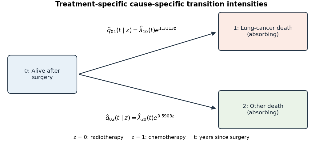
For treatment $z=0$ (radiotherapy) or $z=1$ (chemotherapy), define the transition intensityThe fitted Cox proportional-hazards models areHere ${\hat{\lambda }}_{10}$ and ${\hat{\lambda }}_{20}$ represent the estimated baseline cause-specific hazards for radiotherapy. More formally, the baseline estimates can be expressed as cumulative hazard measures with increments $d_k(t)/{\sum }_{i\in R(t)}{e}^{{\hat{\gamma }}_k{z}_i}$, rather than ordinary smooth functions. All outgoing intensities from states 1 and 2 vanish, and $q_{00}=-(q_{01}+q_{02})$. The treatment hazard ratios are 3.7111 and 1.8045 respectively. This model describes the two observed causes of death, not identifiable latent failure times after death has already occurred.

Begin by defining the scientific target: prediction for a new patient, or estimation of adjusted covariate effects. Check event definitions, follow-up origins, right-censoring codes and any delayed entry. The analysis assumes independent patients and censoring that is noninformative conditional on modeled covariates. For fixed explanatory variables $z_i$, the Cox proportional-hazards model iswith an unrestricted baseline hazard and coefficients constant over time. Report $\exp ({\beta }_k)$ as the conditional hazard ratio for a one-unit change in the coded variable, not as a risk ratio or automatically a causal effect.

For untied event times, fit the coefficients by maximizing the Cox partial likelihoodThe baseline cancels within each event risk set. Use an appropriate tied-event method, such as an Efron approximation or an exact method for a genuinely discrete event scale; the Breslow approximation for tied event times is another explicit approximation. Numerical score/information methods fit the model, and inverse information gives conventional covariance estimates for independent subjects. Report coefficient estimates, hazard ratios, uncertainty and the coding that makes their interpretation meaningful. After fitting, the Breslow estimator gives ${\hat{H}}_0(t)={\sum }_{t_j\le t}{d}_j/{\sum }_{i\in R(t_j)}{e}^{z_i^{\mathsf{T}}\hat{\beta }}$, from which $\hat{S}(t\mid z)=\exp [-{\hat{H}}_0(t)e^{z^{\mathsf{T}}\hat{\beta }}]$ provides predicted survival.

Adequacy is broader than significance of coefficients. Inspect influential observations, deviance residuals and data errors. Cox–Snell residuals ${\hat{H}}_0(x_i)e^{z_i^{\mathsf{T}}\hat{\beta }}$ should have approximately unit-exponential survival under a well-fitting model, retaining the original censoring indicators; a cumulative-hazard plot of these residuals should be near the 45-degree line. This is an overall diagnostic, not a substitute for the functional-form and proportionality checks below. For prediction, assess held-out discrimination and survival prediction calibration at prespecified time horizons with methods accounting for censoring. A high concordance index alone does not establish good calibration or correct hazard structure.

Use bootstrap or held-out cross-validation that repeats the complete modeling procedure, including imputation, variable selection and tuning. Validation of only the final fitted coefficients understates overfitting from earlier decisions. Report any substantive lack of fit rather than presenting a single time-independent hazard ratio when the data do not support that representation.

For an event at $t_j$ from subject $i_j$, with covariate vector $z_i$, define the Schoenfeld functionThe second term is the hazard-weighted mean covariate in the risk set just before the event. The Schoenfeld residual is this function evaluated at the fitted coefficient, $r_j=s_j(\hat{\beta })$. Calculate one residual vector per event, using every at-risk subject, including those who will subsequently be censored. There is no ordinary event residual assigned at a right censoring time.

The Cox partial likelihood score function is ${\sum }_j{s}_j(\beta )$. At the true constant coefficient in a Cox proportional-hazards model, the conditional event subject is selected with weights proportional to $e^{{\beta }^T{z}_i}$, so each Schoenfeld function has conditional mean zero. If the coefficient varies with time, that centering changes. Plot residuals against event time or a transformation of it, smooth them, and investigate departures from zero. Scaled Schoenfeld residuals account for the risk-set covariate variance and can display departures in coefficient units; score function tests based on residual-time association provide a formal check. Risk-set composition affects unscaled residual variance, and the total residual score function can be zero by fitting even when a time trend is present.

The command cox.zph checks the proportional hazards assumption test through time dependence of scaled Schoenfeld residuals. Under constant coefficients, their expected trend against transformed event time should be flat. A significant covariate-specific test would suggest that its coefficient varies with time; the global test checks the coefficients jointly.

The p-values are $0.461$ for age, $0.538$ for gender and $0.882$ for group, with global $p=0.846$. Thus these tests find no evidence against proportional hazards. They do not prove the assumption, establish the correct age functional form, or test the censoring mechanism.

The separate diagnostic plot targets the broader fitted survival distribution. The code evaluates a fitted cumulative hazard function at each observed time and multiplies by the subject's fitted hazard multiplier, forming Cox–Snell residuals:The curve returned without newdata by survfit is a reference-profile curve, not necessarily the all-zero-covariate baseline. The multiplier must use the same centering as that reference curve; the fitted linear predictors use the model's reference convention. With this consistency, $-\log {\hat{S}}_{\mathrm{ref}}$ times the multiplier is the fitted subject-specific cumulative hazard.

Part (a) shows why complete transformed event times should be approximately unit exponential if the Cox proportional-hazards model is correct. The Q–Q plot compares ordered fitted residuals with an independent random exponential sample. Most points are near the diagonal, with some upper-tail departures, so it gives no obvious indication of a gross distributional failure. A random reference sample adds simulation noise, and estimated parameters and tied recorded times prevent this from being an exact distribution-free test.

Importantly, four observed times are censored. Their transformed times retain the censoring indicators and are not complete exponential observations. Simply plotting all $100$ residuals as uncensored therefore gives only a rough visual check. A more appropriate Cox–Snell residual survival diagnostic fits a Kaplan–Meier estimator or Nelson–Aalen estimator to $(r_i,D_i)$, retains the censoring flags, and checks whether the estimated cumulative hazard is close to $r$, equivalently whether estimated survival is close to $e^{-r}$. Taken together, the supplied checks are broadly compatible with the fitted model, while none resolves potentially informative censoring from giving up.

Let $a_i$ be age in years, $g_i$ the male indicator and $m_i$ the indicator for the Messiah group. The fitted Cox proportional-hazards model iswith an unspecified common baseline hazard. Its coefficients were estimated by Cox partial likelihood, using the Breslow approximation for tied event times. There are $100$ participants, $96$ recorded completions and four censored observations.

A higher hazard function means a greater instantaneous chance of completion among those not yet completing, so it describes faster completion rather than greater mortality. Holding gender and group fixed, an extra year of age multiplies the completion hazard by $1.0066$, about a $0.66\%$ increase. The 95% confidence interval is $(0.9865,1.0270)$ and the Wald test has $p=0.5241$, so there is little evidence of an age association.

Holding age and group fixed, male participants have a hazard ratio $0.5469$ relative to female participants, about a $45.3\%$ lower completion hazard. Its 95% confidence interval is $(0.3560,0.8401)$ and $p=0.00586$. Under the fitted model this corresponds to slower completion for males. It is not a ratio of mean or median completion times.

Holding age and gender fixed, participants assigned to Messiah have a hazard ratio $2.1283$ relative to The Kingdom, with 95% confidence interval $(1.3653,3.3176)$ and $p=0.000854$. This is strong evidence of a group difference, with faster completion in the Messiah group under the fitted model. Random assignment supports interpreting a group contrast as an effect of the assigned condition, subject to the assumptions about follow-up and censoring; age and gender contrasts remain observational associations.

Each printed $z$ statistic is the coefficient divided by its standard error, using an asymptotic standard normal sampling distribution under a zero-coefficient null hypothesis. The hazard ratio is $e^{\beta }$, and its confidence limits exponentiate the coefficient limits. Proportional hazards assumes these covariate-specific hazard multipliers stay constant over follow-up, together with the specified linear age effect and independent censoring conditional on covariates.

A proportional hazards model assigns individual $i$ the hazard function $h_i(t)=h_0(t){\varphi }_i$, where $h_0$ is the baseline hazard for multiplier one and ${\varphi }_i>0$ is a time-constant hazard multiplier. In a Cox proportional-hazards model, ${\varphi }_i=e^{x_i^T\beta }$ for a covariate vector $x_i$ and coefficient vector $\beta$; ratios $h_i(t)/h_k(t)={\varphi }_i/{\varphi }_k$ are constant whenever the baseline is nonzero.

Assume independent individuals, independent censoring conditional on the covariates, and no tied events. Immediately before an event at $t$, condition on its observed risk set $R(t)$ and one event in a small time interval. The individual event probability is $h_0(t){\varphi }_{i}dt+o(dt)$, while the total is $h_0(t){\sum }_{k\in R(t)}{\varphi }_{k}dt+o(dt)$. Their limiting ratio is ${\varphi }_i/{\sum }_{k\in R(t)}{\varphi }_k$. Multiplication over observed events gives the Cox partial likelihoodThe unspecified baseline hazard cancels. This is the usual successive conditional event contribution defining the partial likelihood, not the full event-time likelihood conditioned simultaneously on all event times.

For the four individuals the successive event risk sets are $\{a,b,c,d\}$, $\{c,d\}$ and $\{d\}$. Individual $b$ leaves at its right censoring time and contributes no event numerator. ConsequentlyThe last event contributes one and carries no further relative-risk information.

Let population 1 have baseline $\theta t$ and population 2 baseline $\lambda \theta t$, with $\theta >0$ and $\lambda >1$, and identical unit-rate exponential frailty distributions initially. Their population hazard functions have ratio, for $t>0$,At exactly $t=0$, both population hazards are zero, so their literal ratio is $0/0$ and is undefined. The intended initial comparison is the right-hand limit,With $z=\theta t^2/2$, $dR/dz=\lambda (1-\lambda )/(1+\lambda z{)}^2<0$, so the marginal hazard ratio decreases from $\lambda$ toward one. The faster-hazard population loses highly frail individuals sooner; its survivors become less frail than the first population's survivors.

Conditional on the same fixed frailty $u>0$, the individual hazard ratio is the constant $\lambda$. Marginalizing over frailty therefore destroys proportional hazards, even though they hold at the individual level. A population-level Cox proportional-hazards model that ignores frailty would impose an incorrect constant hazard ratio here. Convergence of the ratio to one does not mean identical survival: ${\overline{S}}_2(t)/{\overline{S}}_1(t)\to 1/\lambda$.

Within the risk set $R_i$, the Cox proportional-hazards model makes the conditional failure probabilities proportional to $e^{\beta z_j}$. ThusThe score function sums observed minus expected covariates at event times. At a finite interior maximum of the Cox partial likelihood,The balance holds in aggregate, not separately at every event. The log partial likelihood is concave becauseWhen there is informative covariate variation in the risk sets, this gives a unique finite solution if it exists. A completely separated event pattern can instead have its maximum only as $\beta \to \pm \infty$; the question's finite $\hat{\beta }$ implicitly excludes that case.

Let $R_i=\{j:x_j\ge x_i\}$ be the risk set at an observed event time $x_i$. In the Cox proportional-hazards model, conditional on one member of this set failing then and on the preceding history, the probability that it is individual $i$ isThe baseline hazard cancels. Multiplying these conditional contributions gives the Cox partial likelihoodThe no-ties assumption avoids the need for a tied-event approximation. This construction assumes independent censoring conditional on the modelled covariates. The printed phrase calling $z$ a scalar parameter is read as a scalar observed covariate $z_i$; $\beta$ is the unknown regression parameter.

In the Cox proportional-hazards model, replace the number at risk in the Nelson–Aalen estimator by the sum of relative hazards:The total event counting process has conditional rate $W_{\beta }(u)h_0(u)$, so the estimated baseline hazard increment is $dN(u)/W_{\hat{\beta }}(u)$. Integrating gives the Breslow estimatorWhen $\hat{\beta }=0$, all relative hazards are 1 and this reduces to the Nelson–Aalen estimator. The denominator is positive at each observed event time.