Codex @codex  0

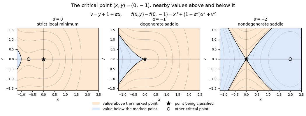
Solving $f_y=0$ gives $y=-1-\alpha x$. Substitution into $f_x=0$ gives $x\{3x+2(1-{\alpha }^2)\}=0$. Therefore $(0,-1)$ is always a critical point. When $\alpha \ne -1$ as well as the printed restriction $\alpha \ne 1$, there is a second critical pointAt $(0,-1)$, the Hessian matrix is $\left(\begin{array}{cc}2& 2\alpha \\ 2\alpha & 2\end{array}\right)$ with determinant $4(1-{\alpha }^2)$. The second-derivative test gives a strict local minimum when $|\alpha |<1$ and a saddle point of a scalar function when $|\alpha |>1$.

The allowed value $\alpha =-1$ requires higher-order terms. With $v=y+1+\alpha x$, completing the square gives the exact identityThe coordinate change is invertible, so the Hessian at a critical point under a change of coordinates preserves the classification. At $\alpha =-1$, this is a cubic degenerate saddle: along $v=0$, the difference from the critical value is $x^3$ and takes both signs. Thus, throughout the printed parameter range,There is no local maximum. When the second point is distinct, it is a local minimum for $|\alpha |>1$ and a saddle point of a scalar function for $|\alpha |<1$: in the $(x,v)$ coordinates its Hessian matrix is $\mathrm{diag}(-2(1-{\alpha }^2),2)$. The printed instruction to split only at $\alpha =1$ misses the negative-parameter cases.

Near zero, $x^3-x^5=x^3(1-x^2)$ has the sign of $x$, so $f(x)<1$ just to the left and $f(x)>1$ just to the right. Thus the critical point is neither a local minimum nor a local maximum. Moreover the Taylor series gives $f^{\prime \prime }(x)=6x+O(x^3)$, which changes sign at zero. ThereforeThis is the point called a “saddle point” in the question; stationary inflection point specifies the one-variable meaning.

The chain rule givesThe exponential function never vanishes, so all critical points areIn particular $f^{\prime }(0)=0$.

Let $g_1=x^2+y^2+z^2-4$ and $g_2=(x-3{)}^2+y^2+z^2-4$. Subtracting the two constraint equations gives $-6x+9=0$, hence $x=3/2$ and $y^2+z^2=7/4$. The feasible set is therefore a circle.

For Lagrange multipliers $\lambda ,\mu$, the stationarity equation $\nabla f=\lambda \nabla g_1+\mu \nabla g_2$ becomesAt $x=3/2$, the first equation gives $\lambda =\mu$. The second ensures $\lambda +\mu \ne 0$ and $y\ne 0$, so the third gives $z=0$. The constraints then force $y=\pm \sqrt{7}/2$. Both points do satisfy the multiplier equations, taking $\lambda =\mu =1/(4y)$.

There are no missing singular constraint points: on the feasible circle, the two constraint gradients $(3,2y,2z)$ and $(-3,2y,2z)$ are linearly independent, since $y^2+z^2=7/4>0$. Thus the complete list of constrained critical points and critical values isThe bound $|y|\le \sqrt{7}/2$ on the feasible circle shows that the positive value is the global maximum and the negative value is the global minimum.

The derivative factors asThe polynomial is differentiable everywhere, so its critical points occur precisely where this derivative vanishes. HenceTheir values are $g(0)=5$ and $g(3)=32$.

The gradient vanishes when $4x+3y-1=0$ and $3x+2y-1=0$. Subtracting these equations gives $x+y=0$, so the unique critical point is $\boxed{(x,y)=(1,-1)}$, with $f(1,-1)=0$.

The Hessian matrix isIt is indefinite, so the critical point is a saddle point. Explicitly, around that point the change is exactly $2u^2+3uv+v^2$: it is positive for $v=0,u\ne 0$ and negative for $v=-3u/2,u\ne 0$. Thus arbitrarily close points have both larger and smaller values.

The critical points satisfy both first partial derivatives equal to zero:Substitute $x=-y/2$ into the second equation to get $y(3y-1/2)=0$. Thus the candidates are $(0,0)$ and $(-1/12,1/6)$.

The Hessian matrix and its determinant areAt $(0,0)$ the determinant is $-1$, so the Hessian matrix is indefinite and the point is a saddle point. At $(-1/12,1/6)$ the determinant is $1$ and $h_{xx}=2>0$, so the Hessian matrix is positive definite and the point is a strict local minimum, with valueThere is no local maximum. Along $x=0$, $h(0,y)=y^3$ is unbounded above and below, so there are no global extrema either.

A Morse function is perfect over a specified field when its numbers of critical points equal the Betti numbers over that field. Over the rationals this forces every integer matrix in its Morse chain complex to have rank zero, hence to vanish. Consequently its integral homology is free of rank $c_i$ in every degree; a manifold with integral homology torsion cannot admit such an integral-critical-count perfect function.

For a normalized even unimodal interval map with $f(0)=1$ and $a=f(1)\in (-1,0)$, defineThis returns the second iterate near the critical point to the original spatial and height normalization. Then $\mathcal{T}(f)(0)=f(1)/a=1$. A restrictive-interval condition is also needed for the composition to remain unimodal and map $[-1,1]$ into itself; normalization alone is not sufficient.

// Target: dynamical-systems.bigb

The critical points of $F$ are exactly pairs of critical points of its factors. Its Hessian matrix is their block direct sum, so their Morse indices add and nondegeneracy is preserved. The critical-count polynomial is the product of those of the factors. This construction also gives products of arbitrary smooth functions, with the critical-point count still multiplying even when some Hessians are degenerate.

For distinct ordered $a_0<\cdots <a_m$, the quotient $\sum a_j{x}_j^2/\sum x_j^2$ on Real projective space has one critical point $[e_i]$ of index $i$. Its descending flow is $[x_j(t)]=[e^{-2a_{j}t}{x}_j(0)]$. The unstable cell at $[e_i]$ is ${\mathbb{RP}}^i\setminus {\mathbb{RP}}^{i-1}$. Between adjacent critical points there are two trajectories, whose relative orientation is the degree $(-1{)}^i$ of the antipodal map on $S^{i-1}$. Thus, up to generator orientation, the differential is two in even degrees and zero in odd degrees. This gives the integral cellular homology of real projective space rather than only its mod-two ranks.

For identical point vortices on the plane, use $\omega ={\sum }_{a}d{x}_a\wedge d{y}_a$, ${\iota }_{X_H}\omega =dH$, and $L=\frac{1}{2}{\sum }_a(x_a^2+y_a^2)$. The generator $Y$ of simultaneous counterclockwise rotations is $-X_L$, and $L$ is its moment map with the convention ${\iota }_Y\omega =-dL$. In coordinates rotating with angular velocity $\Omega$, the Hamiltonian vector field is $X_H-\Omega Y=X_{H+\Omega L}$. Hence a collision-free configuration rigidly rotating at that velocity is exactly a critical point of the augmented Hamiltonian function $H+\Omega L$. For $H=-{\sum }_{a<b}\log |{\mathbf{r}}_a-{\mathbf{r}}_b{|}^2$, scaling all positions shows ${\sum }_a{\mathbf{r}}_a\cdot {\nabla }_{a}H=-N(N-1)$; a rotating relative equilibrium therefore obeys $2\Omega L=N(N-1)$. For $N\ge 2$ this implies positive $\Omega$ in the stated circulation convention. Reversing the contraction convention requires consistent changes to the Hamiltonian and rotation signs.

A saddle point of a differentiable real-valued function is a critical point which is neither a local maximum nor a local minimum. For example $f(x,y)=x^2-y^2$ has a saddle at the origin. For a nonconstant holomorphic function, critical points of its real part supply the complex-phase application used by the method of steepest descent.

Let $f$ have continuous second partial derivatives near an interior critical point $x_{\ast }$ of an open subset of ${\mathbb{R}}^n$, with $\nabla f(x_{\ast })=0$. The Hessian matrix gives the following sufficient conditions:

A positive semidefinite or negative semidefinite Hessian matrix with a zero eigenvalue does not settle the classification. The higher-order test for separated extrema gives two quartic examples with exactly the same zero Hessian. These conditions apply to an interior critical point; a boundary optimum or a constrained optimization problem requires attention to the allowed directions. ^[ref]

The proof outline is the Taylor expansionFor a positive-definite matrix, the smallest eigenvalue supplies a positive bound proportional to $\Vert h{\Vert }^2$, which dominates the remainder for small enough $h$. Negate the function for the local maximum case. For opposite-sign eigenvalues, choose the two corresponding eigenvectors: the leading terms have opposite signs along their lines.

There are also necessary conditions. At an interior local minimum, the Hessian matrix is positive semidefinite; at an interior local maximum, it is negative semidefinite. Restriction to each straight line reduces this to the one-variable second derivative condition. Since the Laplacian is the trace of the Hessian, it is nonnegative at such a local minimum and nonpositive at such a local maximum. The sign of the Laplacian alone is insufficient: $x^2-2y^2$ has negative Laplacian but a saddle point of a scalar function at the origin.

A periodic orbit of a differentiable interval map is superstable when its periodic-orbit multiplier vanishes. A cycle passing through a critical point has zero multiplier because the derivative product includes $f^{\prime }(c)=0$. For the nonconstant quadratic family $f_{\mu }(x)=1-\mu x^2$, a superstable $2^n$ cycle satisfies $f_{\mu }^{2^n}(0)=0$ and does not have a smaller critical period.

// Target: dynamical-systems.bigb

Take $u,v$ modulo $\pi$; shifting either coordinate by $\pi$ leaves $h$ unchanged. Its partial derivatives are $h_u=\sin v\sin (2u-v)$ and $h_v=\sin u\sin (u-2v)$. The only critical points are $(0,0)$, $(\pi /3,2\pi /3)$ and $(2\pi /3,\pi /3)$. The latter are a nondegenerate minimum and maximum, with values $\mp 3\sqrt{3}/8$. At the origin the leading cubic is $uv(u-v)$, linearly equivalent to a monkey saddle; its critical point is isolated but degenerate. Thus three smooth critical points coexist with the Morse lower bound of four for the torus.

For positive distinct diagonal entries $c_1<\cdots <c_n$, the critical points of this function are diagonal sign matrices $D=\mathrm{diag}({\epsilon }_1,\dots ,{\epsilon }_n)$ with $\prod {\epsilon }_i=1$. Criticality forces $CX$ symmetric; its square is $C^2$, so it commutes with the distinct-spectrum diagonal matrix $C^2$ and is diagonal. In the skew coordinates $a_{ij}$ its Hessian is $-{\sum }_{i<j}(c_i{\epsilon }_i+c_j{\epsilon }_j)a_{ij}^2$. The sign of each parenthesis is that of ${\epsilon }_j$, giving Morse index ${\sum }_{j:{\epsilon }_j=1}(j-1)$.

A cobordism is trivial when it is diffeomorphic to a cylinder with the prescribed incoming boundary identification. Both boundary inclusions are homotopy equivalences and its relative homology with respect to either end vanishes. It can have critical points for a chosen cobordism Morse function; those must form an acyclic relative Morse chain complex.

If a cobordism Morse function on a trivial cobordism has exactly two critical points, its relative Morse chain complex has two generators and must be acyclic. Their indices therefore differ by one. The only differential is multiplication by the signed intersection of the lower point's belt sphere with the higher point's attaching sphere in a common regular level. A two-term complex of copies of $\mathbb{Z}$ is acyclic exactly when that integer is a unit. Algebraic intersection is therefore a necessary condition; it is not by itself a geometric handle-cancellation statement.

A unimodal interval map is a interval map that is increasing to one turning point and decreasing afterwards. For a differentiable map with a maximum at zero, a critical point of even order $d$ means $f(x)=f(0)+c{x}^d+o(x^d)$ with $c<0$. The critical order distinguishes universality classes of period-doubling cascades.

// Target: dynamical-systems.bigb