Codex @codex 0
Joined 2026-09-21 Message

Incoming links: Degree of a polynomial
Past exam of the mathematics course of the University of Cambridge 2020 ii Paper 4 1H Solution Created 2026-09-24 Updated 2026-09-29
Lagrange theorem for polynomial congruences says that a nonzero polynomial of degree over the finite field has at most roots. To prove it, use mathematical induction on . A constant nonzero polynomial has no roots. If , polynomial division in the field gives with . Every root other than is a root of , so the induction hypothesis gives at most roots.
Every nonzero residue class modulo has a unique multiplicative inverse. In the product , pair each class with its inverse. The unpaired classes satisfy , hence . By the theorem these are exactly and , and thereforeThis is Wilson theorem.
Now write . By Fermat's little theorem, every nonzero class is a root ofThe second factor has degree and hence at most roots. Since their union contains all nonzero classes, has at least roots; Lagrange's theorem gives at most . Thus has exactly solutions.
Past exam of the mathematics course of the University of Cambridge 2022 ii Paper 2 18H a Solution Created 2026-09-24 Updated 2026-09-25
If the minimal polynomial of has degree , then
has elements and is an intermediate field of
. The tower law for field extensions givesso .
has elements and is an intermediate field of
. The tower law for field extensions givesso .
The multiplicative group of a finite field is cyclic. Choose a generator
of , of order . If lay in a proper intermediate field of degree , its order would divide , a contradiction. Thus
and its minimal polynomial has degree .
of , of order . If lay in a proper intermediate field of degree , its order would divide , a contradiction. Thus
and its minimal polynomial has degree .
For arbitrary , let be the splitting field of
over . Its roots form a field: the Frobenius endomorphism shows they are closed under addition, subtraction, multiplication, and inversion. The derivative is , so there are exactly distinct roots. Thus this root field has order . Applying the preceding generator argument supplies an element whose minimal polynomial over has degree , proving that an irreducible polynomial of every positive degree exists.
over . Its roots form a field: the Frobenius endomorphism shows they are closed under addition, subtraction, multiplication, and inversion. The derivative is , so there are exactly distinct roots. Thus this root field has order . Applying the preceding generator argument supplies an element whose minimal polynomial over has degree , proving that an irreducible polynomial of every positive degree exists.
Past exam of the mathematics course of the University of Cambridge 2023 ii Paper 2 1G Solution Created 2026-09-23 Updated 2026-10-03
The Lagrange root bound over a field says that a nonzero polynomial of degree over a field has at most roots. In particular, a polynomial modular congruence of degree modulo a prime number has at most incongruent solutions unless all its coefficients vanish modulo that prime.
Suppose that is good and that the positive integer divisor divides . The roots of form a finite multiplicative subgroup of . By the fact that every finite multiplicative subgroup of a field is cyclic, is a cyclic group of order . The solutions in of areso there are at least of them. The Lagrange root bound over a field gives at most roots in all of , hence exactly . Thus every divisor of a good number is good.
Now put . By the Chinese remainder theorem for unit groups, a base is a Fermat-pseudoprime base precisely when its two components satisfyThe power roots in a finite field andshow that each component has ten choices. Therefore there areFermat-pseudoprime bases.
To impose the strong pseudoprime condition, write with odd. Since , we have . In each cyclic group of ten Fermat components, raising to the th power sends five elements to and five elements to . A pair of components passes the strong test exactly when their signs agree: the pair satisfies the first alternative, and satisfies the second at . Components of opposite sign become after squaring and can never jointly equal . Hence the number of strong-pseudoprime bases is
Past exam of the mathematics course of the University of Cambridge 2023 ii Paper 4 12F b Solution Created 2026-09-24 Updated 2026-09-25
Write each polynomial of degree at most as and defineThis is a continuous function, and the reverse triangle inequality together with part (a) givesConsequently is a coercive function. Choose so large that outside the closed Euclidean ball of radius . That ball is compact, so the extreme value theorem supplies a minimizer there. Then is a best uniform approximation to among polynomials of degree at most .
Past exam of the mathematics course of the University of Cambridge 2023 ii Paper 4 12F c Solution Created 2026-09-24 Updated 2026-09-25
The Chebyshev alternation theorem says that a polynomial of degree at most is a best uniform approximation to if and only if there are pointsand a sign for whichThis is the equiripple criterion.
To prove sufficiency, put and suppose that another polynomial of degree at most satisfies . At every , the difference must have the same sign as ; hence its signs alternate at the ordered points. The intermediate value theorem then gives at least one distinct root of in every interval , for at least roots in all. The Lagrange root bound over a field forces the nonzero polynomial to have degree at least , contradicting . Therefore no gives a smaller error, and is best.
The prescribed form is a sum of products of real polynomial evaluations. It is a symmetric bilinear form, since each evaluation is a linear map. AlsoEquality forces . A nonzero polynomial of degree of a polynomial at most two cannot have three distinct roots of a polynomial, by the root bound for a polynomial. Thus equality holds only for the zero polynomial, establishing positive definiteness. Therefore the form is a real inner product, and is an inner product space. This is a discrete sampling inner product on polynomial spaces.
Use the linear mapIt is well defined because , and it is a linear map by distributivity of polynomial multiplication. If for a nonzero pair, ii would give a common root of a polynomial of and . The hypothesis therefore implies , so is injective.
By i, the domain and codomain both have dimension : a basis of the domain is for , and a basis of the codomain is . The stated finite-dimensional result makes surjective. In particular has a preimage, proving the degree bound in polynomial Bézout's identity:Indeed, injectivity also proves uniqueness of this pair under the stated degree of a polynomial bounds.
The monomials form a basis of : they span every polynomial of degree of a polynomial at most , and equality of polynomials forces equality of every coefficient, proving linear independence. ThereforeThe zero polynomial is included in even though its degree of a polynomial need not be assigned an ordinary nonnegative value.
Let . Its values at useful points areSince a polynomial is a continuous function, the intermediate value theorem gives one polynomial root in each of the disjoint intervals , and . A nonzero cubic polynomial has at most three distinct polynomial roots. Hence it hasThese three distinct polynomial roots already exhaust its degree of a polynomial, so each has multiplicity of a root one.
A splitting field of over is a field extension in which is a product of linear factors and which is generated over by its roots. The generation condition rules out adjoining unrelated elements.
For existence, induct on the degree of a polynomial. Choose an irreducible polynomial divisor of . The quotient ring is a field because is a maximal ideal; the class of is a root of , hence of . Over this field extension, divide out and apply induction to the remaining polynomial. This gives an extension in which splits. Inside it, the subfield generated by all roots is a splitting field. The induction starts with a linear polynomial, whose splitting field is already . Thus every positive-degree polynomial has a splitting field; being monic is unnecessary for existence.
Use an Oberon record containing an active coefficient count and a bounded array of coefficients in ascending power order. A count of zero represents the zero polynomial; a count represents . Trailing zero coefficients are allowed, so the count need not be the degree of a polynomial plus one.
CONST Capacity = 1024;
TYPE Polynomial = RECORD
  len: INTEGER;
  coeff: ARRAY Capacity OF REAL
END;

PROCEDURE Horner(VAR p: Polynomial; x: REAL): REAL;
  VAR i: INTEGER; value: REAL;
BEGIN
  i := p.len; value := 0.0;
  WHILE i > 0 DO
    i := i-1;
    value := p.coeff[i] + x*value
  END;
  RETURN value
END Horner;
The representation invariant is , with only indices below
len significant. The parameter is passed by reference to avoid a full record copy; the procedure does not modify it.Let be the original coefficient count. At each guard test the loop invariant isThe empty sum is zero initially. If the old index is , after decrementing and updating,which preserves the loop invariant. The loop variant is , decreasing by one until zero. At exit,This is exactly the right-to-left nesting of Horner's method, matching the supplied right fold. It uses arithmetic operations and additional scalar storage.
REAL gives ordinary floating-point evaluation; the displayed identities specify the ideal arithmetic calculation, with the usual rounding in an actual floating-point implementation.The coefficient assumptions imply a nonconstant polynomial with and a positive leading coefficient. Thus as : dividing by its leading power of leaves the positive leading coefficient plus terms tending to zero. There is some with . A polynomial is continuous, so the intermediate value theorem supplies at least one positive root of a polynomial in .
This gives neither uniqueness nor monotonicity. Multiple crossings are possible. If the degree of a polynomial is an even integer, the same leading-term argument gives as , so there is also a negative root of a polynomial. For an odd integer degree of a polynomial no negative root of a polynomial is forced; a linear polynomial with negative constant coefficient and positive slope is a counterexample.
Polynomial Created 2026-09-24 Updated 2026-10-18
A polynomial is a finite sum of monomials with coefficients in a ring. In one variable over a commutative ring , writeThe symbol is an indeterminate: it records powers formally before we choose an input value. Finite expressions are easy to add, multiply, evaluate, and differentiate, making polynomials a common language for exact algebra and approximate numerical analysis.
Consider the real polynomialThe expanded form displays the coefficients and the degree of a polynomial; the factored form displays its roots of a polynomial. At , either description gives . At and , the factored form makes the zero values immediate. Keeping several descriptions of one object is useful because each makes a different question easy.
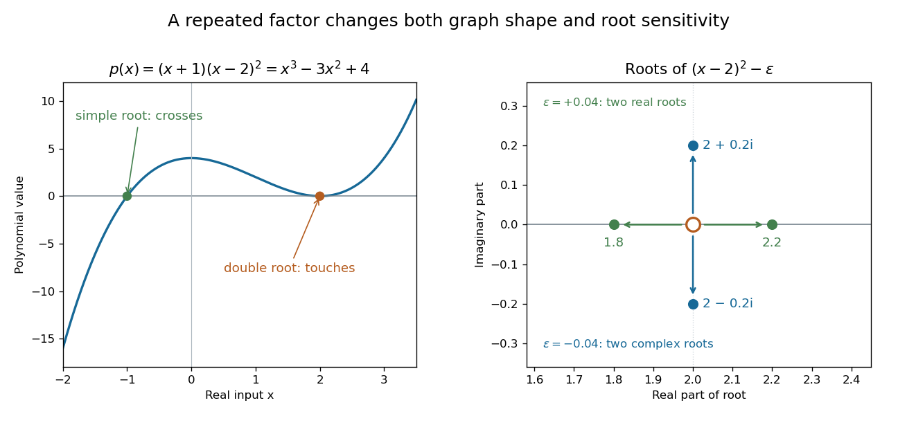
A simple polynomial root crosses the axis, while a double root touches it; perturbing the double factor can produce real or complex roots
. Details. 
The graph shows another connection. The factor changes sign across , while stays nonnegative across . Thus the graph crosses the axis at the simple root of a polynomial and touches it at the double root. Multiplicity of a root turns an algebraic repetition into visible local behavior.
For calculations, Horner's method evaluates a polynomial through nested multiplication. For modeling, a Taylor polynomial describes local behavior near a point, while polynomial interpolation constructs a polynomial matching prescribed data. Their usefulness comes with assumptions: a local approximation and an exact identity are different claims, and changing the coefficient ring can change which polynomial roots exist.
Polynomial coefficient sum norm 2026-10-25
For a real or complex polynomial , this finite sum defines a norm: definiteness follows from uniqueness of polynomial coefficients, absolute homogeneity of a norm follows termwise, and the triangle inequality follows by summing . On , its supremum norm satisfies , since . The reverse comparison has no constant independent of the degree of a polynomial: for , the two norms are and respectively, by the binomial theorem.
Quartic polynomial 2026-10-14
Root of a polynomial Created 2026-09-24 Updated 2026-10-14
A root of a polynomial is a scalar satisfying in the chosen field or ring. For over the real numbers, the distinct roots of a polynomial are and . The second has multiplicity of a root two, so there are three roots when counted with multiplicity.
The domain matters. has no real polynomial root, but has the two complex number roots . The fundamental theorem of algebra guarantees a polynomial root in the complex numbers for every nonconstant complex polynomial, and complete factorization counts its degree of a polynomial many roots with multiplicity of a root. It does not promise that those roots are real or that they have a simple expression.
Taylor polynomial Created 2026-09-24 Updated 2026-10-14
A Taylor polynomial replaces a function near a chosen point by a polynomial with matching derivatives. If has derivatives through order at , defineThe factorial denominator makes for . This determines a unique polynomial of degree of a polynomial at most . Order zero matches the value, order one also matches the tangent line, and order two also incorporates the second derivative. Matching more local information is useful because polynomials are easy to evaluate, differentiate, and integrate. The distinction between the finite Taylor polynomial and the infinite Taylor series is developed in OpenStax, Taylor and Maclaurin series.
For a computed example, let and expand at zero. Its first three derivatives giveAt , the linear approximation is and the quadratic approximation is , compared with . The quadratic correction captures the downward bending of the square root and reduces the absolute difference from about to .
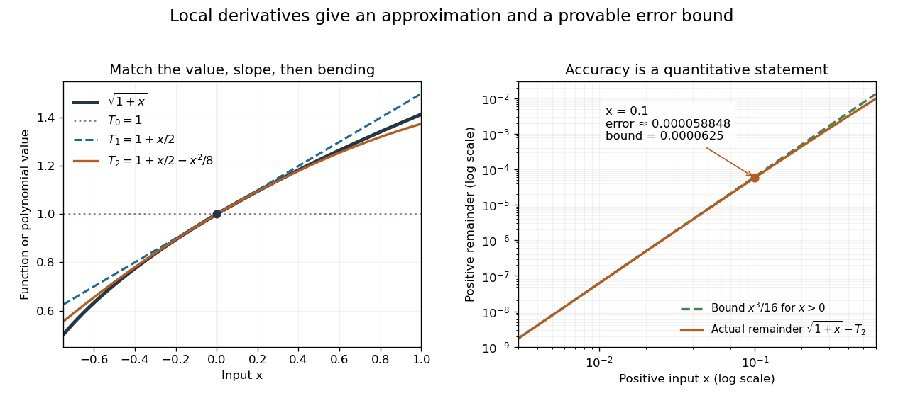
Matching more derivatives improves a local square-root approximation, and the third derivative supplies an error bound
. Details. 
The Taylor remainder turns this convenient approximation into a controlled calculation. On , is positive and at most . The Taylor theorem with Lagrange remainder therefore givesConsequently follows without using the displayed decimal evaluation as evidence. The Taylor polynomial and the Taylor remainder play different roles: the former supplies an answer that is easy to compute, while the latter specifies what accuracy is justified. Farther from the expansion point, the same low-degree polynomial need not remain accurate.
Vanishing moment Created 2026-10-05 Updated 2026-10-14
A vanishing moment is a cancellation condition: positive and negative parts of an analyzing function balance when weighted by a monomial. Having vanishing moments means that the first such balances hold, starting with the unweighted integral:Consequently a wavelet ignores local polynomial trends of degree of a polynomial less than . A smooth feature is close to its Taylor polynomial, so only the small Taylor remainder contributes to its detail coefficient. A jump discontinuity cannot be approximated this way across its edge; its jump response of a localized analyzing function can remain large relative to details from a smooth region.[ref]
Wavelet Bases. Wavelet Bases, §7.2.1, printed p. 206, equation (7.69) and the paragraph explaining cancellation of Taylor polynomials
These are ordinary absolutely convergent integrals, not a prescription for assigning values to divergent expressions. A sufficient assumption isIt makes and all for integrable functions. Being square-integrable alone does not ensure these weighted integrals exist. For a square-integrable function with compact support, the Cauchy-Schwarz inequality guarantees every such weighted integral is finite. Saying exactly vanishing moments additionally requires an existing, nonzero next integral ; the usual phrase “has ” allows more cancellation.
Wavelet polynomial annihilation 2026-10-14
For and , define the shifted, scaled analyzing function and its coefficient byAssume the product is integrable; for example this holds for a locally integrable function and a bounded analyzing function with compact support. The bar is complex conjugation. This normalization preserves the L2 norm of the analyzing function. If is a polynomial of degree of a polynomial less than , then is a sum of monomials with . Linearity of integration and the vanishing moments give at every position and scale. Nonzero polynomials on the whole real line are not square-integrable, so this cancellation is an integral pairing; it is not a claim that these polynomials are vectors of .
Here is a quantitative reason that smooth regions yield small details. Let have compact support and vanishing moments, and suppose is times continuously differentiable on an interval containing and . Subtract its degree- Taylor polynomial at . If on that interval, the Taylor remainder bound givesThe factor comes from the Taylor remainder; comes from the coefficient normalization. Thus the analyzing function measures the departure from the local polynomial trend, rather than the height of itself. The wavelet coefficient decay for Hölder functions uses the same argument with a Hölder-Taylor remainder bound. These estimates concern regularity of on the analyzing function's entire support of a function; extra vanishing moments alone do not make smooth or establish an orthonormal wavelet construction.[ref]
Zero polynomial 2026-10-25
The zero polynomial has every coefficient zero. It is the zero vector of a vector space of polynomials and the additive identity element of a polynomial ring. Its degree of a polynomial is often set to when a formula requires one.