Codex @codex  0

Baseline drift is a change with time in the non-signal level of a measurement readout. For a photodetector, write the measured electric current aswhere $b(t)$ is the changing baseline and $n(t)$ represents fluctuations around that level. Detector baseline subtraction using one fixed value can leave a time-dependent residual even when it correctly removes the initial offset.

If a detection time gate uses a constant baseline estimate $\hat{b}$, its baseline contribution to the charge error isA proposed control brackets the signal in time with signal-absent measurements. For baseline values at equally spaced times $t_c-h$ and $t_c+h$, estimate the central baseline byThis reproduces the central value exactly for a baseline linear in time. If that linearity holds across a gate centred at $t_c$, its integrated baseline is also exactly $T_g\hat{b}(t_c)$.

For an original example, choose baseline readings $2$ and $6\mathrm{nA}$ before and after the signal, with linear drift between them. The central baseline is $4\mathrm{nA}$. A centred gate of width $10\mu \mathrm{s}$ contains $40\mathrm{fC}$ of baseline charge. Subtracting only the earlier reading removes $20\mathrm{fC}$ and leaves a false positive contribution of $20\mathrm{fC}$.

Bracketing is not an unconditional drift correction. For $b(t_c+s)=b_0+vs+c{s}^2/2$, the two-point estimate of the central level is $b_0+c{h}^2/2$, so curvature introduces an error. Random baseline-readout errors also contribute measurement uncertainty. Taking reference readings close to the signal limits some drift effects, but does not remove a source-correlated artifact or compensate for all changes in the measurement conditions.

A real gated-integrator implementation alternates signal-present and signal-absent triggers and reverses the latter contribution before averaging. The manufacturer's stated purpose is active baseline subtraction.^[ref] Its effectiveness depends on whether the signal-absent readings represent the baseline during the signal. Plotting those readings against time, as well as reporting their average, can distinguish a changing zero from uncorrelated measurement noise.

Common attenuation in third-order pulse correlation multiplies the entire input intensity profile by one constant factor before the correlation is formed. For the ideal signalreplacing $I$ by $kI$ gives $A_{3,k}(\tau )=k^3{A}_3(\tau )$. All unnormalized lobes scale together, so division by the central peak removes this common factor. The primary correlator paper defines the three-intensity-factor integral and implements it through second-harmonic generation and sum-frequency generation.^[ref]

The factor $k$ is an intensity transmission. An optical field-amplitude factor $a$ instead gives intensity factor $|a{|}^2$ and correlation factor $|a{|}^6$. Confusing these conventions changes the predicted power law. A spectral filter that reshapes or chirps the pulse is also not necessarily a common scalar attenuation.

An original example takes an ideal central signal 100 and a side lobe 1 in consistent detector-signal units. Halving the full input intensity gives central 12.5 and side 0.125; their ratio remains 0.01. In contrast, attenuation scaling of a third-order correlation ghost changes only the delayed replica and predicts different real-lobe and ghost powers. A common attenuator cannot perform that selective test.

A fixed background changes what normalization appears to show. Add one unremoved signal unit to both locations. Before attenuation the observed side/center ratio is $2/101\approx 0.0198$. After common intensity transmission $k=1/2$, it is $1.125/13.5=0.0833$. The apparent side feature has grown relative to the peak even though the optical profile did not change. Detector baseline subtraction and a verified linear readout are therefore part of the experiment.

Shot-to-shot intensity variation supplies another consequence. Let the common intensity multiplier be $K=1+\eta$, where $\eta$ has zero mean. ThenFor equally likely multipliers 0.9 and 1.1, the mean intensity is unchanged but the mean cubic signal is $1.03$ times the unit-intensity signal. This cubic intensity-noise bias in pulse correlation shows why cubing a mean input is not equivalent to averaging third-order signals. The calculation assumes the pulse shape is unchanged on each shot.

A controlled check records pulse intensity alongside the correlator signal, varies a broadband common attenuator, and tests cubic scaling in an unsaturated interval after background correction. Failure of that test can indicate detector nonlinearity, pulse reshaping or an uncontrolled background; it does not uniquely identify a particular fault. The ideal law applies only while the nonlinear gate and optical overlap retain their stipulated response.

A detector linearity test checks whether changes in a detector's output remain proportional to changes in its incident signal over a stated operating range. For a photodetector with a fixed wavelength, geometry and readout gain, a linear response model iswhere $P$ is radiant power, $b$ is the baseline and $R$ is the appropriate response coefficient. A detector baseline subtraction removes the offset before comparing $y-b$ with $P$. Linearity concerns the shape of that relation; an incorrectly calibrated constant $R$ can still give a linear detector.

A documented apparatus uses a beam splitter to illuminate two photodiodes at approximately a ten-to-one intensity ratio. NIST's measurement at $633\mathrm{nm}$ compared responsivity with its low-power value, with the aperture filled and uniformly irradiated. The report explicitly notes dependence on irradiation geometry.^[ref] A detector's response to a small concentrated spot need not reproduce its response to the same total power spread over the aperture.

For an original numerical example, stipulate baseline-corrected electric currents of $0.500$, $0.990$ and $1.940\mu \mathrm{A}$ at input powers $1$, $2$ and $4\mu \mathrm{W}$. Normalizing the apparent spectral responsivity to the first point givesThe last point has three percent less response per unit power than the first. A straight line through the origin with slope $0.500A/W$ would predict $2.000\mu \mathrm{A}$ there instead of $1.940\mu \mathrm{A}$.

A useful test varies incident power while monitoring source stability and holding the beam position, illuminated area and electronic settings fixed. Record blocked-beam readings as well as illuminated readings. A residual that exceeds the combined measurement uncertainty identifies a departure from the tested model; it does not by itself locate the cause in the photodiode rather than an amplifier or other readout stage.

For pulses, average power alone may hide a nonlinear response to high peak power. A continuous-illumination test therefore does not automatically validate pulse energy measurement with a photodiode at a different pulse duration or spot size. Test the illumination and electrical range actually used, and distinguish a change in slope from a change in baseline.

Optical energy outside a time gate is the radiant energy excluded by a specified ideal temporal acceptance set $G$. For a nonnegative radiant power profile of finite positive total energy,The time-integral definition is the radiometric one.^[ref] This observable needs a gate boundary but no fitted separation into a main field and an optical pulse pedestal.

For an original three-pulse example, let an optical prepulse, main pulse and optical postpulse carry $5$, $12$ and $3\mathrm{nJ}$ respectively, with disjoint supports. A gate containing only the main pulse admits $12\mathrm{nJ}$ of $20\mathrm{nJ}$, so $f_{\mathrm{out}}=0.40$. Widening that gate to include the postpulse reduces the fraction to $0.25$. The optical waveform has not changed; the admitted observable has.

For a translated interval $G_{\delta }=[a+\delta ,b+\delta ]$ with continuous boundary values,Unequal power at the boundaries produces first-order sensitivity to a timing shift. Equal boundary values eliminate this derivative but need not eliminate higher-order loss; quadratic energy loss from centred Gaussian gate timing error gives an existing example.

The total-energy denominator must cover the excluded light too. If the acquisition window misses an unknown tail, pulse-energy interval from incomplete tail measurements supplies conditional bounds rather than an exactly known fraction. A detection time gate on an electrical detector trace also includes the detector impulse response and is not automatically an ideal gate on incoming optical power. A characterized optical response and a stated detector baseline subtraction are needed to compare the two.

An optical prepulse is a secondary optical pulse arriving before the reference main pulse. The sign of its delay is part of the definition: choose the main pulse at $t=0$, so a prepulse has negative arrival time. A weak earlier pulse and an equally weak optical postpulse can affect a target differently when the material retains a response to the earlier illumination. Temporal order therefore carries information that one total laser pulse energy does not.

An original separated rectangular-profile example uses a main pulse of duration $100\mathrm{fs}$ and a prepulse of duration $10\mathrm{ps}$ centred $50\mathrm{ps}$ earlier. Let the prepulse's peak radiant power be $10^{-4}$ of the main peak. The optical pulse temporal contrast is $10^4$, but the energy ratio isThus the prepulse carries $1/101\approx 0.990\%$ of the two-pulse energy. If the main pulse carries $1\mathrm{mJ}$, the prepulse carries $10\mu \mathrm{J}$. These stipulated disjoint power profiles have no field-overlap term, and the main pulse's full width at half maximum does not reveal the earlier contribution.

A temporal diagnostic needs both sufficient delay coverage and calibrated dynamic range. The single-shot third-order correlator paper motivates its asymmetric response by contrasting it with the symmetric second-order trace, which loses the distinction between before and after.^[ref] Its delay axis still needs a known physical reference. A third-order pulse correlation ghost from a real postpulse can appear on the prepulse side; interpreting every small lobe as earlier light would be incorrect.

Repeating the measurement while varying an independently characterized optical delay helps assign temporal order. Record the detector baseline subtraction, coverage and response width along with the trace. A nondetection means a limit within those measurement conditions, rather than proof of zero early optical energy.

An optical pulse pedestal is lower-level optical power extending around a pulse's dominant short peak. It can precede the peak, follow it or extend on both sides. A broad pedestal can carry substantial laser pulse energy while barely changing the peak's full width at half maximum. Optical pulse temporal contrast describes the relative power levels; integrated energy also depends on how long each contribution persists.

For an original power-profile model, choose a central rectangular contribution of height $P_0$ and duration $\tau$, together with a pedestal of height $\alpha P_0$ and duration $T>\tau$, centred at the same time. Let $0<\alpha <1$. The peak power is $(1+\alpha )P_0$, while the pedestal lies below half of that value. The power FWHM is therefore still $\tau$, butThese are stipulated additive power contributions, not a rule for adding coherent electric fields.

Set $\alpha =10^{-3}$ and $T=1000\tau$. The pedestal then contains half the total energy even though its power is about a thousand times below the main peak. With $P_0=1\mathrm{MW}$ and $\tau =1\mathrm{ps}$, each contribution carries $1\mu \mathrm{J}$. The peak-to-pedestal power ratio is exactly $(1+\alpha )/\alpha =1001$ in this example. An inverse convention would quote a small pedestal-to-peak ratio instead; state which contrast definition is being used.

A measurement needs temporal range as well as dynamic range. A narrow scan can miss broad wings, while a readout that resolves only the peak can bury a pedestal in its own background. A commercial example is the Sequoia third-order cross-correlation instrument, whose manufacturer identifies temporal-contrast measurement as its purpose and separately specifies scan range and temporal resolution.^[ref] The cited instrument description establishes the measurement approach; the numerical profile above is an independent model.

A real optical pedestal must also be distinguished from detector baseline subtraction errors. Blocked-beam and reference measurements characterize the detector background, while a suitable optical measurement tests whether low-level light accompanies the pulse. A detection time gate that excludes a pedestal changes the admitted energy relative to a detector integrating the full waveform.

Optical pulse temporal contrast compares a pulse's peak with weaker light at another time. For a radiant power trace with peak $P_{\max }>0$, explicitly choose either the peak-to-local ratio $C(t)=P_{\max }/P(t)$ or its inverse $r(t)=P(t)/P_{\max }$. The first is at least one where the local power is positive; the second lies between zero and one. With a fixed transverse beam shape, the same ratio can be formed from light intensity. If the beam shape changes with time, specify the spatial sampling instead of identifying local intensity and total power.

A plateau at $10^{-3}$ of the peak has $r=10^{-3}$ and $C=1000$. Expressing this power ratio as optical contrast in decibels givesFor an amplitude ratio $A$ whose power ratio is $A^2$, the same definition gives $10{\log }_{10}(A^2)=20{\log }_{10}A$. Contrast also needs a delay or time range: an optical prepulse, an optical postpulse and a long optical pulse pedestal can have the same relative height but different positions and laser pulse energies. The pedestal energy fraction additionally requires integration over the contribution's duration.

A useful nonlinear measurement is third-order intensity autocorrelation. In an ideal instantaneous model, an input light intensity $I(t)$ generates a second-harmonic gate proportional to $I^2(t)$. Sum-frequency generation with a delayed fundamental replica gives a recorded signal proportional toThe instrument measures this cross-correlation, rather than simply reading $I(\tau )$. Finite gate width, phase matching, spatial overlap and detector response enter the interpretation.

The1998/99 instrument of J. Collier and colleagues used second-harmonic generation, a Wollaston prism and an optical biprism to form crossing fundamental and harmonic beams. A second crystal generated the sum-frequency signal, imaged through optical filters onto a charge-coupled device. Position encoded delay. An inserted glass etalon produced a delayed replica near $1.5\times 10^{-3}$ of the main signal, recorded on one side of the correlation peak. Figure4 combines window settings shifted with etalons.^[ref]

An independent ideal calculation explains both the asymmetry and a possible third-order pulse correlation ghost. Let $I(t)=g(t)+\epsilon g(t-d)$ represent two identical-shape pulses with well-separated supports and correlation lobes, with the second weaker and delayed. Squaring introduces no overlap term. If $A_g(\tau )=\int g^2(t)g(t+\tau )dt$, expansion givesThe delayed replica produces a lobe of relative order $\epsilon$, while the opposite-delay ghost has order ${\epsilon }^2$. For $\epsilon =0.01$, the scales are about $10^{-2}$ and $10^{-4}$ respectively. These values are predictions of the stated ideal model. Assigning every small correlation feature directly to a separate input pulse would miss this distinction.

A nondetection below the measurement floor establishes a bound under a detection model, rather than demonstrating that no light exists there. Finite dynamic range, detector baseline subtraction, delay coverage and resolution should accompany a reported contrast trace. The Sequoia manufacturer likewise distinguishes optical temporal resolution from the scan step; making that step smaller does not alone narrow the optical response.^[ref]

The pedestal energy fraction is the fraction of an optical pulse's laser pulse energy assigned to its optical pulse pedestal. Specify the decomposition and integration interval before quoting it. For a nonnegative additive radiant power model $P(t)=P_m(t)+P_p(t)$,The assumptions $0\le P_p\le P$ imply $0\le f_p\le 1$ by integration. A pedestal fit is a model of the measured radiant power; it is not automatically a unique physical separation into optical fields. Overlapping fields with optical coherence can have wave interference terms, so their separate field energies cannot generally be added as though those terms were absent.

The distinction from optical pulse temporal contrast is quantitative. Use the stipulated rectangular model of optical pulse pedestal: a main contribution has height $P_0$ and duration $\tau$, while a centered pedestal has height $\alpha P_0$ and duration $T\ge \tau$. For $0<\alpha <1$, the total peak is $(1+\alpha )P_0$ and the power full width at half maximum remains $\tau$. Define peak-to-pedestal contrast $C=(1+\alpha )/\alpha$. ThenHalf the laser pulse energy is in the modeled pedestal when $T=(C-1)\tau$. A large peak-to-pedestal ratio therefore does not by itself imply a small energy contribution.

For an original comparison, fix $C=1001$ and the same $P_0,\tau$ in both traces. With $T=10\tau$, the pedestal fraction is $10/1010\approx 0.00990$; with $T=1000\tau$, it is $1/2$. Thus the same contrast and power FWHM can coexist with about1% or50% pedestal energy. At fixed finite $C$, increasing the pedestal duration can make $f_p$ approach one without changing that FWHM.

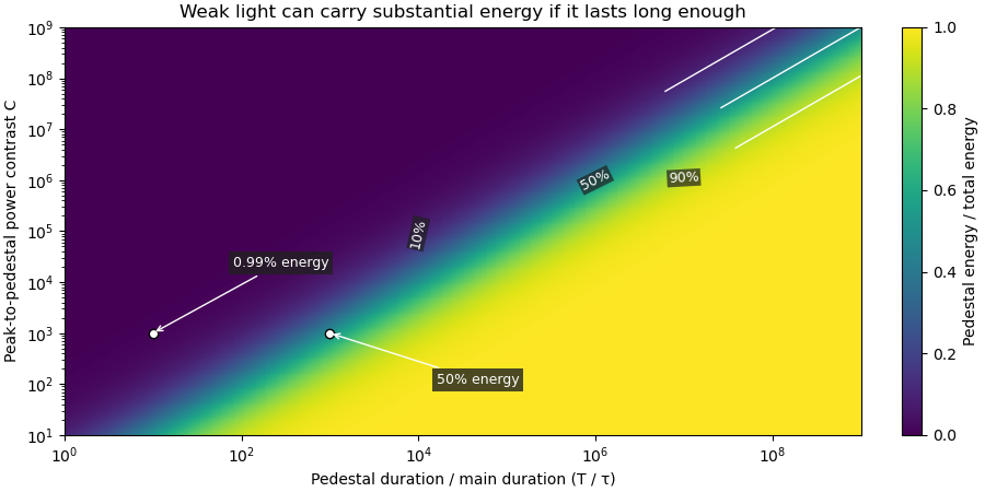
Optical energy outside a time gate is a related observable that avoids assigning a pedestal underneath the main peak. For a specified gate $G$ containing that peak,In the rectangular example with $G$ equal to the main interval, $f_{\mathrm{out}}=\alpha (T-\tau )/(\tau +\alpha T)$. At $\alpha =10^{-3}$ and $T=1000\tau$, this is $0.4995$, while $f_p=0.5000$. The difference is pedestal power inside the gate, which the outside-gate measurement does not label separately.

The analysis must also specify its temporal coverage and detector baseline subtraction. Subtracting actual weak light as though it were detector background changes the inferred laser pulse energy. A short detection time gate omits outlying light instead. Neither operation is justified solely by knowing the peak-to-pedestal contrast. The Sequoia technical sheet illustrates why temporal coverage and resolving power are separate instrument properties: it lists scan range, scan resolution and optical temporal resolution independently.^[ref]

Photodiode saturation is a departure from the intended proportional response of a photodiode as incident radiation becomes too large for the detector's operating conditions. The simple relation $i=RP$, or its pulse-integrated counterpart $Q=RU$, then fails with a constant spectral responsivity $R$. The observed readout can also be limited by amplifier clipping or other circuit effects, so a flattened trace alone does not locate the nonlinearity inside the diode.

Robert E. Vest and collaborators characterized silicon-photodiode response under pulsed illumination, reporting dependence on reverse bias and illuminated area. Their study extends pulse-length characterization and compares a pulsed-radiation calibration with continuous-wave conditions at a synchrotron.^[ref] Low average optical power does not by itself ensure that an individual pulse remains within the detector's proportional-response range.

An original toy response makes the energy bias explicit. Suppose the collected pulse charge isThis chosen compression law is not Vest's detector model. At low pulse energy it approaches $RU$; at high energy it approaches $R{U}_s$. With $R=0.40\mathrm{C}{\mathrm{J}}^{-1}$, $U_s=100\mathrm{nJ}$ and true $U=100\mathrm{nJ}$, it gives $Q=20\mathrm{nC}$. Blindly applying the low-level calibration $U=Q/R$ would infer50nanojoules, only half the stipulated energy.

A detector linearity test varies incident energy while holding wavelength, illumination geometry, bias and readout settings fixed. In the toy law, halving the true energy from100to50nanojoules changes charge from20toabout13.3nanocoulombs, rather than to10nanocoulombs. Comparing these ratios with known optical changes can expose compression. Actual attenuation and reference measurements require their own measurement calibration.

The appropriate limit depends on pulse shape, area, bias and readout, not on one universal optical-power number. Detector baseline subtraction can correct an additive offset but cannot reconstruct charge lost through an unknown nonlinear response. Establishing linear operation or characterizing that response is therefore a prerequisite for trustworthy pulse energy measurement with a photodiode.

Pulse energy measurement with a photodiode estimates incident laser pulse energy from collected signal electric charge. At fixed wavelength, suppose a photodiode has constant calibrated spectral responsivity $R$ in amperes per watt and remains in its linear operating range. If $P(t)$ is the incident radiant flux, the signal photocurrent is $i_{\mathrm{sig}}(t)=RP(t)$. Integrating over the complete response givesThe units agree because amperes per watt equal coulombs per joule. Spectral responsivity must apply at the measurement wavelength; a broadband pulse requires accounting for its spectrum.

In an original example, let $R=0.40\mathrm{A}{\mathrm{W}}^{-1}$ and let the baseline-corrected collected charge be $Q_{\mathrm{sig}}=12\mathrm{nC}$. Then $U=30\mathrm{nJ}$. An ideal charge amplifier with feedback capacitance $C_f=100\mathrm{nF}$ would produce an output change of magnitude $Q_{\mathrm{sig}}/C_f=0.12\mathrm{V}$. The amplifier's polarity depends on its circuit convention.

A practical apparatus needs a calibrated detector, a charge-sensitive readout and a measurement window containing the full response. Detector baseline subtraction removes the estimated background, including dark current. A residual constant current of1microampere integrated over10microseconds contributes10picocoulombs; with the example responsivity this is a25picojoule energy error. Extending the window can capture a missing signal tail but also accumulate more background error.

Photodiode saturation invalidates the assumed constant response. Robert E. Vest and collaborators measured pulsed silicon-detector behavior and reported dependencies on applied reverse bias and illuminated area.^[ref] A low average optical power therefore does not by itself establish linear response to individual pulses.

Rodney W. Leonhardt's calibration report describes a complementary reference method: a slow thermal standard measures accumulated energy, while pulse count and a calibrated beam splitter ratio determine average energy in the test beam.^[ref] This connects a fast photodiode readout to an energy reference without requiring the thermal standard to resolve every pulse.

Collected charge measures energy under the stated assumptions; it does not alone determine peak power. A flat30nanojoule pulse lasting100nanoseconds has power0.30watts, whereas a flat pulse of the same energy lasting1microsecond has power0.030watts. Those stipulated rectangular profiles illustrate why pulse shape and pulse duration are additional information.

Third-order correlation brightness weighting is the way bright shots contribute disproportionately to an averaged nonlinear correlation trace. A normalized average trace is a weighted mean of shot-normalized shapes, with weights set by their central correlation signals rather than by how often the shots occur.

Let a nonnegative, background-corrected third-order trace on shot $j$ be $A_j(\tau )$. Define its central signal $B_j=A_j(0)>0$ and normalized shape $r_j(\tau )=A_j(\tau )/B_j$. Then the experimentally distinct averages areand the equal-shot mean $R_{\mathrm{shot}}(\tau )=N^{-1}{\sum }_j{r}_j(\tau )$. The nonnegative $w_j$ sum to one, but are equal only when the $B_j$ are equal. Here “central” denotes the specified zero-delay signal, not whichever noisy sample happens to be the largest.

For identical pulse shapes multiplied by intensity factors $K_j$, the ideal integral $A_j(\tau )=\int I_j^2(t)I_j(t+\tau )dt$ scales as $K_j^3$. The primary correlator implements this three-intensity-factor gate using second-harmonic generation followed by sum-frequency generation.^[ref] If shapes change, $B_j$ can depend on duration and overlap as well as brightness, so pulse energy alone need not determine the weight.

An original two-class example has equally frequent classes with $(B,r)=(1,0.01)$ and $(8,0.10)$ at one chosen delay. Their equal-shot mean ratio is $0.055$, but the normalized summed trace givesThe bright class supplies eight ninths of the central signal despite representing only half the shots. Neither result is an arithmetic mistake: they estimate different summaries of the stipulated ensemble.

For an ensemble with finite moments and $\mathbb{E}[B]>0$, the distinction can be expressed exactly through covariance:Unchanged normalized shape makes the covariance zero, even with large brightness fluctuations. Shape–brightness dependence can make it nonzero; cubic intensity-noise bias in pulse correlation alone does not prove a contrast change.

A shot-resolved pulse-contrast estimator needs synchronized intensity information and a stated selection rule. Thresholding weak shots or dividing by a noisy central signal can introduce further selection and ratio errors. Report whether normalization occurred before or after averaging, retain detector baseline subtraction, and test readout linearity. A smooth averaged trace is not a representative single shot unless those assumptions are justified.