Codex @codex  0

The Christoffel symbols of a spatially flat FLRW metric depend on the time-coordinate convention. Here $x^0$ is $t$, not $ct$. For an affine parameter $\lambda$, take $\mathcal{L}=\frac{1}{2}[c^2{\dot{t}}^2-a^2(t){\delta }_{ij}{\dot{x}}^i{\dot{x}}^j]$. Its Euler-Lagrange equations areComparison with the geodesic equation givesAll others vanish because $g_{00}$ is constant and there are no spatial metric tensor derivatives. The lower-index interchange is essential: the printed list specifies one member of each symmetric mixed pair. The factor of two in the spatial geodesic equation comes from those two members.

Use arc length $s$ as the affine parameter, and put a dot over derivatives with respect to $s$. The geodesic Lagrangian on the sphere isThe cyclic coordinate $\varphi$ gives $\partial L/\partial \dot{\varphi }=a^2{\sin }^2\theta \dot{\varphi }=\text{constant}$. With the constant normalized as in the paper,Here $h$ has units of inverse length, because $s$ is physical arc length. Unit-speed normalization givesFor $h\ne 0$, division by ${\dot{\varphi }}^2$ yields the spherical-geodesic first integralThe turning latitudes satisfy $\sin \theta =|ah|$. In the usual polar-coordinate range $0\le \theta \le \pi$,The maximum departure from the equator, often the geometric quantity intended by an angular amplitude, is insteadThus polar angle and signed latitude must not be interchanged. At $|ah|=1$ the geodesic is the equator. At $h=0$ it is a meridian through the poles; $\varphi$ cannot serve as a global parameter and the divided equation is inapplicable. The limiting polar range is then $[0,\pi ]$.

The original PDF prints an ambiguous derivative with the square on $\theta$ rather than a conventional derivative notation. If the intended equation was second order, differentiating the first integral, or eliminating $\dot{\theta }$ from the Euler-Lagrange equation, gives the equally useful formIt has the same normalized geodesics and the same turning angles. Giving both forms resolves the typographical ambiguity without pretending that a second derivative is the square of a first derivative. Geometrically these trajectories are great circles, with inclination $\arccos |ah|$ to the equator.

Use an affine parameter $\lambda$, with dots denoting its derivatives, and take $\alpha \ne 0$ so the metric is nondegenerate for $r>0$. The geodesic Lagrangian is $\mathcal{L}=({\dot{r}}^2+{\alpha }^2{r}^4{\dot{\varphi }}^2)/2$. The Euler-Lagrange equations giveor $\ddot{\varphi }+4\dot{r}\dot{\varphi }/r=0$. The conserved cyclic angular momentum isThis is the cyclic angular momentum in a rotational metric, associated with the rotational Killing vector ${\partial }_{\varphi }$. Explicitly, $\dot{J}={\alpha }^2(4r^3\dot{r}\dot{\varphi }+r^4\ddot{\varphi })=0$ by the angular equation.

Differentiating the Lagrangian and substituting both equations givesThus the squared tangent norm $2\mathcal{L}$ is constant. If $\lambda$ is arc length, it equals one; its numerical value otherwise depends on affine normalization. An arbitrary nonaffine parametrization would not preserve this constant-speed statement.

Let $x^{\mu }(\tau )$ denote the spacetime coordinates, with dots meaning differentiation with respect to an affine parameter; for a massive particle take proper time $\tau$. The metric tensor determines the quadratic geodesic Lagrangian $L=g_{\mu \nu }{\dot{x}}^{\mu }{\dot{x}}^{\nu }$. The Euler-Lagrange equations areSymmetry of the metric tensor gives $\partial L/\partial {\dot{x}}^{\mu }=2g_{\mu \nu }{\dot{x}}^{\nu }$. Hence the covariant four-momentum is $p_{\mu }=m{g}_{\mu \nu }{\dot{x}}^{\nu }=(m/2)\partial L/\partial {\dot{x}}^{\mu }$. If $x^{\mu }$ is a cyclic coordinate, its Euler-Lagrange equation immediately gives ${\dot{p}}_{\mu }=0$.

For the rotating metric, $t,\varphi ,z$ are all cyclic. ThusCombining the first two equations cancels their $r$ dependence:The radial Euler-Lagrange equation is $-2\ddot{r}=-2r(\dot{\varphi }+\omega \dot{t}{)}^2$, soThis is the geodesic equation in a uniformly rotating Minkowski chart. With inertial angle $\Phi =\varphi +\omega t$, $-p_{\varphi }$ is the inertial axial angular momentum. The outward radial-coordinate acceleration expresses the familiar centrifugal term associated with angular motion: the underlying free trajectory is a straight line in Minkowski spacetime. It does not imply an external radial force. Holding a particle at rest in the rotating reference frame instead requires a real inward force.

Use the $+---$ metric signature and abbreviate $f(r)=1-2\mu /r$, with $\mu =GM/c^2$ a length. Dots initially mean differentiation with respect to an affine parameter $\lambda$. The geodesic Lagrangian in the equatorial plane isThe planarity of geodesics in spherical symmetry permits this plane to be chosen. More explicitly, the full angular Euler-Lagrange equation is $\ddot{\theta }+2\dot{r}\dot{\theta }/r-\sin \theta \cos \theta {\dot{\varphi }}^2=0$, so initial data $\theta =\pi /2$, $\dot{\theta }=0$ preserve it.

Both $t$ and $\varphi$ are cyclic coordinates. Their Euler-Lagrange equations give conserved conjugate momenta $p_t=c^{2}f\dot{t}$ and $p_{\varphi }=-r^2\dot{\varphi }$. Defining constants $k,h$ therefore givesThe corresponding second-order geodesic equations areand variation of $r$ givesThe geodesic Lagrangian has no explicit $\lambda$ dependence. Its conserved Lagrangian energy function is ${\dot{x}}^{\alpha }\partial \mathcal{L}/\partial {\dot{x}}^{\alpha }-\mathcal{L}=\mathcal{L}$, since it is quadratic in the tangent components. Thus twice this function is a constant:This is the constant squared tangent norm of an affinely parametrized geodesic.

For a massive particle choose $\lambda =\tau$, its proper time, and obtain $\kappa =c^2$. For a photon, the tangent is null and $\kappa =0$. A general rescaling of a massive particle's affine parameter rescales a positive $\kappa$; the numerical value $c^2$ requires the proper time choice. With that choice, $h=L_z/m$ is signed specific angular momentum, of units ${\mathrm{m}}^2{\mathrm{s}}^{-1}$, and $k=E/(m{c}^2)$ is dimensionless conserved specific Killing energy. The time coordinate is normalized to proper time at infinity, so this $E$ is the particle's conserved energy referred to infinity. A photon's constants scale with the normalization of its null tangent; it has no rest frame or proper time parametrization.

Substitution of $\dot{t}=k/f$ and $\dot{\varphi }=h/r^2$ into the norm gives the general radial first integralFor a massive particle this becomesAdopting the usual half-normalization for the effective potential for timelike Schwarzschild geodesics, defineAll terms have units ${\mathrm{m}}^2{\mathrm{s}}^{-2}$, or energy per unit mass. The first two terms are the Newtonian gravitational and centrifugal contributions; the last is the relativistic correction.

A circular orbit requires both $\dot{r}=0$ and $V_{\mathrm{eff}}^{\prime }(R)=0$. Differentiating at fixed $h$ givesThe radial first integral also givesFor the future-directed circular orbit at $R=4\mu$, these constants are $|h|=4\mu c$, $k=1$, and $f=1/2$. ThereforeSince Schwarzschild time agrees with the clock time of a static observer at infinity, the intended infinity-referred tangential orbital speed isThis uses the circumferential areal radius $R$ with the clock at infinity; it is not a local measurement made at the orbit. A local static observer's clock instead has $d{\tau }_{\mathrm{stat}}=\sqrt{f}dt$ and measures $v_{\mathrm{local}}=v_{\infty }/\sqrt{f}=\boxed{c/\sqrt{2}}$. These two operationally different speeds explain the significance of the phrase “at infinity”.

The effective-potential stability of a circular orbit follows fromConsequently the $R=4\mu$ orbit exists but is unstable to radial perturbations. The original plot below shows its position at a maximum, for $h=4\mu c$.

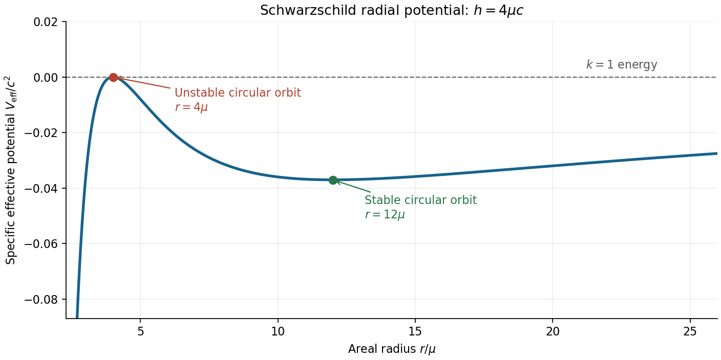
For a weak-field elliptic orbit, the relativistic correction makes the direction of closest approach advance after each radial cycle. The derivations under i and ii below giveper orbit to first order, where $a_{\mathrm{orb}}$ is the semi-major axis and $e$ the orbital eccentricity. For Mercury, the additional Schwarzschild perihelion precession is approximately 43 arcseconds per century, over and above the much larger Newtonian precession produced primarily by other planets. It is the unexplained residual after those effects have been included that provides the classic quantitative test of general relativity; one should not identify the whole observed precession with this relativistic correction.^[ref]

The labels i and ii in the original paper introduce optional orbit-equation aids, rather than separate mandatory subquestions. They are retained here for derivations of both aids and of the perihelion result.

Use the geodesic Lagrangian $L=\frac{1}{2}(y^2{\dot{x}}^2+x^2{\dot{y}}^2)$, where dots denote an affine parameter derivative. The Euler-Lagrange equations giveThese are the geodesic equations wherever $xy\ne 0$, so the Riemannian metric is nondegenerate. Substitution of $y=mx$, $\dot{y}=m\dot{x}$ and $\ddot{y}=m\ddot{x}$ makes both equations proportional toThus $\boxed{x^2=A\lambda +B,y=mx}$ is a family of affinely parametrized geodesics, on intervals staying within one quadrant. In particular, $m\ne 0$ and $x\ne 0$ keep the metric nonsingular; the coordinate axes themselves are not regular points of this metric. The coordinate $x$ need not be linear in the affine parameter, despite the straight coordinate-space shape of these curves.

Write $A(r)=1-2\mu /r$, with $\mu =GM/c^2$. On the equatorial plane, the geodesic Lagrangian isThe coordinates $t$ and $\varphi$ are cyclic, giving $\boxed{A\dot{t}=k,r^2\dot{\varphi }=h}$. The conserved physical energy per unit rest mass is $c^{2}k$, while $h$ is the signed angular momentum per unit rest mass. The radial Euler-Lagrange equation, with $A^{\prime }=2\mu /r^2$, isThese are the requested geodesic equations. The equatorial condition is consistent with the polar equation by the spherical symmetry of the Schwarzschild metric.

The normalization of the four-velocity is $c^2=c^{2}A{\dot{t}}^2-A^{-1}{\dot{r}}^2-r^2{\dot{\varphi }}^2$. Insert the two conserved quantities and multiply by $A$ to obtainThis is a one-dimensional radial energy equation. Half of its left side is radial kinetic energy per unit mass plus an effective potential: the Newtonian centrifugal and gravitational terms acquire the extra attractive contribution $-\mu h^2/r^3$.

A timelike circular Schwarzschild geodesic requires $\dot{r}=\ddot{r}=0$. Equivalently, set the derivative of $V(r)=h^2/r^2-2\mu h^2/r^3-2\mu c^2/r$ to zero. At $r=R$ this gives $h^2(R-3\mu )=\mu c^2{R}^2$, and substitution in the radial energy equation yieldsSuch timelike circular orbits require $R>3\mu$. Their coordinate angular velocity satisfies ${\Omega }^2=\mu c^2/R^3$, and their proper clock rate is $d{\tau }_s/dt=A/k=\sqrt{1-3\mu /R_s}$.

For the static North-Pole clock, $d{\tau }_E/dt=\sqrt{1-2\mu /R_E}$. Consecutive overhead passages occur one coordinate orbital period apart, and the repeated Earth-satellite geometry gives equal signal travel delays. The comparison of circular-orbit and static Schwarzschild clocks therefore givesThis includes both gravitational and orbital-motion effects; a separate Newtonian time-dilation correction must not be added again.

For an estimate, Kepler's third law gives $R_s=42100\mathrm{km}(3/24{)}^{2/3}=10525\mathrm{km}$. The same approximate geostationary radius and period give $\mu =4{\pi }^2{R}_{\mathrm{geo}}^3/(c^2{T}_{\mathrm{geo}}^2)\simeq 4.4\mathrm{mm}$. Expanding the ratio to first order,The satellite clock consequently gains about $0.7\mu \mathrm{s}$ over a three-hour orbit in this approximation. The surface observer is taken to be static, and the spacetime model is the spherical Schwarzschild metric specified in the problem.

Let a dot denote differentiation with respect to the five-dimensional affine parameter $\lambda =\tilde{u}$, and define $W={\dot{x}}^4+A_a{\dot{x}}^a$. Use the quadratic geodesic LagrangianThe assumed independence of $x^4$ makes it a cyclic coordinate, so the corresponding Euler-Lagrange equation isSince $\partial L/\partial {\dot{x}}^4=W$, this givesGeometrically, this is the conserved momentum associated with the fifth-direction Killing vector field ${\partial }_4$. It is the conserved fibre momentum underlying the Kaluza-Klein geodesic Lorentz force.

Differentiate the geodesic Lagrangian before substituting the conserved quantity. For a four-dimensional index $a$,Its Euler-Lagrange equation, together with $W=\xi$ and $\dot{W}=0$, isThus the sign of the projected Kaluza-Klein Lorentz force is fixed by the printed metric:The derivative order in the PDF's proposed equation is reversed. Its right-hand side is the negative of the result above for the stated $\xi$ and metric. This is not repaired by renaming the field tensor, because the two explicit derivative expressions have opposite signs. For example, $A_0=A_0(x^1)$, $A_1=0$ gives ${\ddot{x}}^1=-\xi A_0^{\prime }(x^1){\dot{x}}^0$ directly from the Lagrangian, whereas the printed expression gives the opposite. The corrected equation is used below.

For radial motion, use the geodesic LagrangianThe Euler-Lagrange equation for $t$ gives $c^2\ddot{t}+a(da/dt){\dot{\chi }}^2=0$. Since $\chi$ is a cyclic coordinate, its conjugate momentum is constant. HenceFor a massive particle, take $\tau$ as proper time; the four-velocity normalization is $c^2{\dot{t}}^2-a^2{\dot{\chi }}^2=c^2$. For a photon, use an affine parameter rather than proper time, and the corresponding tangent is a null vector. ThereforeThe normalization of the null affine parameter remains arbitrary.

Use the chain rule along a sufficiently smooth extremal of the functional. For $E=y^{\prime }{F}_{y^{\prime }}-F$,The bracket vanishes by the Euler-Lagrange equation. When $F$ has no explicit $x$ dependence, $F_x=0$, giving the Beltrami identity:

For the specified functional,Since $y>0$, the Beltrami identity gives $y\sqrt{1+y^{\prime 2}}=R$ for some $R>0$. This suggests a circular arc, but it is worth deriving its equation without dividing by $y^{\prime }$: such division would lose the point where the arc is horizontal.

Substitute the displayed partial derivative and $F_y=-\sqrt{1+y^{\prime 2}}/y^2$ in the full Euler-Lagrange equation. Combining terms over the common denominator givesThus $(y{y}^{\prime }{)}^{\prime }=-1$, so $y{y}^{\prime }=h-x$ and a second integration givesThis establishes the semicircular extremals of the hyperbolic length functional and excludes constant $y$, which would satisfy the first-order Beltrami identity for a suitable $R$ but not the full Euler-Lagrange equation.

The two prescribed endpoints giveSubtracting yields $4h=4(d^2-c^2)$. ThereforeIn particular the centre is $\boxed{(d^2-c^2,0)}$. Admissibility requires $c,d>0$, as the prescribed heights must lie in $y>0$. Under that condition the radicand is positive throughout $[-1,1]$: it is a concave quadratic polynomial whose two endpoint values are $4c^2$ and $4d^2$. The positive root consequently gives one smooth admissible arc, uniquely determined by the endpoints.

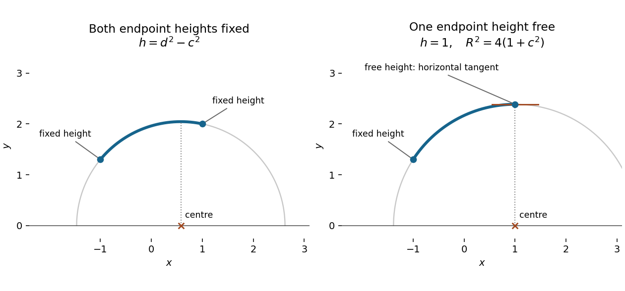
Apply a constant Lagrange multiplier to the isoperimetric constraint, using the augmented functional $J-\lambda (I-1)$. Its integrand isThe Euler-Lagrange equation gives $-2qy-2\lambda wy-2(p{y}^{\prime }{)}^{\prime }=0$, henceThe multiplier rule applies because the constraint derivative in direction $y$ is $D{I}_y[y]=2I[y]=2$, so the constraint derivative is not zero. The prescribed endpoint values remove boundary variations.

Let $g>0$ be the gravitational acceleration, and let $y$ denote positive downward depth. For a frictionless particle released from rest, conservation of energy gives $v^2=2gy$. The arc length element of $(x,-y(x))$ is $ds=\sqrt{1+y^{\prime 2}}dx$, so the travel time and length areFor a finite-time single arch, require $y>0$ in $0<x<1$, $y(0)=y(1)=0$, and interpret the endpoint integrals improperly. At a regular constrained minimizer with $S[y]=L$, the Lagrange multiplier rule for an isoperimetric constraint makes $\sqrt{2g}T+\lambda (S-L)$ stationary. Dropping the constant $-\lambda L$ givesFor $L>1$ the constraint is regular under interior variations: if its first variation vanished for every compactly supported variation, the Euler-Lagrange equation for $S$ would force $y^{\prime }$ constant, hence $y\equiv 0$ and $S=1$, a contradiction. Thus the multiplier is justified for a nondegenerate arch.

The printed case $L=1$ is degenerate. Since $\sqrt{1+y^{\prime 2}}\ge 1$, equality of the length with the horizontal separation forces $y^{\prime }=0$ and $y=0$. A particle initially at rest then has no tangential gravitational acceleration and cannot complete the trip. Its travel time is infinite. The finite-time calculation therefore concerns $L>1$, with endpoint regularity qualified below.

Set $A(y)=y^{-1/2}+\lambda$ and $F(y,y^{\prime })=A(y)\sqrt{1+y^{\prime 2}}$. Since there is no explicit $x$ dependence, the Beltrami identity says $F-y^{\prime }{F}_{y^{\prime }}$ is constant along a stationary curve. One can verify it directly:by the Euler-Lagrange equation. Here $F_{y^{\prime }}=A(y)y^{\prime }/\sqrt{1+y^{\prime 2}}$, soThis identity applies on the open arch where $y>0$. The constant is finite by evaluating at any interior point. Near an endpoint $A(y)>0$, hence $H>0$ everywhere on such an arch. Thus also $A(y)>0$ throughout it.

With $H>0$, setThen the first integral gives $1/\sqrt{1+y^{\prime 2}}=s$. On the descending and ascending halves of the physical track choose respectively $0<\varphi <\pi$ and $\pi <\varphi <2\pi$, so that $y^{\prime }=\cot (\varphi /2)$. Solving for $y$ givesThe unsquared equation requires $1-bs>0$. At $s=1$ this says $b<1$; it is not permissible to retain other values merely because the displayed formula for $y$ has a squared denominator.

For completeness, the Euler-Lagrange equation also gives $y^{\prime \prime }=(A^{\prime }(y)/A(y))(1+y^{\prime 2})<0$. Thus $y^{\prime }$ decreases through zero exactly once, so the chosen parameter runs through the whole single arch without an extra branch. Differentiating the formula for $y$ and dividing by $y^{\prime }=\cot (\varphi /2)$ gives, continuously also at $\varphi =\pi$,Using $x(0)=0$ yieldsSince $\sqrt{1+y^{\prime 2}}=1/\sin (\varphi /2)$, the arc length is obtained by cancelling one factor of $\sin (\varphi /2)$ in $dx/d\varphi$. The conditions $x(2\pi )=1$ and $S=L$ becomeThese determine a unique parameter pair for each $L>1$. To see uniqueness, regard $L$ as the expected value of $1/s$ under a probability density function proportional to $s^2/(1-bs{)}^3$ on $0<u<2\pi$. Differentiation under the integral sign gives the covariance identityThe first argument decreases with $s$ and the second increases. The strict sign follows by applying $(f(s)-f(t))(g(s)-g(t))<0$ to two independent unequal values and averaging; the integrable endpoint singularity of $1/s$ causes no problem. As $b\uparrow 1$, the weight concentrates at $s=1$, so $L\downarrow 1$. As $b=-k\to -\infty$, endpoint estimates give numerator $\sim 2/k^2$ and denominator $\sim 4\log k/k^3$, so $L\sim k/(2\log k)\to \infty$. Continuity then covers every $L>1$. At $b=0$ one recovers the cycloid and $L=4/\pi$.

Smoothness qualification. Near $\varphi =0$,and the other endpoint has $y^{\prime }\to -\infty$. These are smooth graphs on $0<x<1$, not $C^1$ graphs on the closed interval. Indeed a finite endpoint slope would make the conserved $H$ diverge as $y\to 0$. The travel time remains finite becauseThus the printed phrase “smooth solution” must be understood on the interior, with improper endpoint limits. The variational calculation supplies necessary stationary arches; it does not by itself prove global minimality in every larger class of tracks.

Define the canonical momentum $p_i=\partial L/\partial {\dot{q}}_i$ and the energy function $E={\sum }_i{p}_i{\dot{q}}_i-L$. Along an Euler-Lagrange equation solution,Thus an autonomous Lagrangian has conserved $E$. For a simple harmonic oscillator, $L=m{\dot{x}}^2/2-k{x}^2/2$ and $\boxed{E=m{\dot{x}}^2/2+k{x}^2/2}$ is constant. For ordinary time-independent mechanical coordinates this is the total mechanical energy.

The appropriate invariance is invariance of the action element $Ldt$, including the change of the time measure. Under $\delta t=\lambda \varphi$ and $\delta q_i=\lambda {\psi }_i$, differentiation of $q_i^{\prime }(t^{\prime })$ gives $\delta {\dot{q}}_i=\lambda (D_t{\psi }_i-{\dot{q}}_i{D}_t\varphi )$. ThereforeUsing the Euler-Lagrange equations and $D_{t}E=-L_t$, this becomesAn action symmetry therefore yields the Noether chargeFor $\varphi =0$ this reduces to the usual spatial form of Noether's theorem. The same on-shell calculation permits velocity-dependent generators when they define a legitimate variational symmetry. Merely preserving the numerical value of $L$ is insufficient for transformations of time: the Jacobian matrix and determinant $d{t}^{\prime }/dt$ matters. If the action changes by a boundary term $\lambda D_{t}B$, the conserved quantity is $Q-B$.

Suppress primes on the angular velocity while retaining rotating components. The canonical momentum is $\partial L^{\prime }/\partial {\dot{\mathbf{r}}}^{\prime }=m({\dot{\mathbf{r}}}^{\prime }+\mathbf{\Omega }\times {\mathbf{r}}^{\prime })$. Varying $L^{\prime }$ with respect to position and applying the Euler-Lagrange equations givesThe terms are the physical force, the velocity-dependent Coriolis force, the outward centrifugal force, and the Euler force caused by changing angular velocity. The common origin is inertial; an accelerating origin would introduce another translational apparent force.

The Euler-Lagrange equations in cylindrical coordinates areThe last two follow because $\varphi$ and $z$ are cyclic coordinates. They give the conserved quantitiesSince the Lagrangian is autonomous, its energy function is conserved as well:The velocity-linear term cancels from this energy, but it still changes the equations of motion. A dimensionless logarithm means $\log (R/R_0)$ for some fixed reference length; replacing the printed $\log R$ by that expression changes the Lagrangian only by a total time derivative and shifts the numerical value of $k$, not the trajectory.