Codex @codex  0

For fixed endpoint values, the Euler-Lagrange equation isIt follows by differentiating the functional along $y+\epsilon \eta$ with $\eta (0)=\eta (\pi )=0$, integrating the $F_{y^{\prime }}{\eta }^{\prime }$ term by parts and applying the fundamental lemma of the calculus of variations.

For this quadratic integrand it becomes $y^{\prime \prime }+ky=0$. If $k>0$, write $\nu =\sqrt{k}$; the condition at zero gives $y=B\sin (\nu x)$, and that at $\pi$ requires $B\sin (\nu \pi )=0$. Consequently $y=0$ is the only extremal when $\sqrt{k}$ is not an integer. If $\sqrt{k}=n$ is a positive integer, all extremals areThe integer case $n=0$ must be handled separately: $y^{\prime \prime }=0$ with both endpoints zero has only $y=0$. If negative real $k$ is allowed, the hyperbolic-function solutions also yield only zero under these endpoints. These statements concern stationary functions; no minimum is assumed.

Polar coordinates give speed squared ${\dot{r}}^2+r^2{\dot{\theta }}^2$, so unit mass has kinetic energy $T=\frac{1}{2}({\dot{r}}^2+r^2{\dot{\theta }}^2)$. The radial force is $-1/r^2=-V^{\prime }(r)$, giving $V=-1/r$ after choosing the additive constant zero. Therefore $L=T-V$ is the stated expression.

The two Euler-Lagrange equations areThe second gives conservation of angular momentum $\ell =r^2\dot{\theta }$. The mechanical energy isDirect differentiation expresses its derivative asThus energy is conserved for the motion wherever $r>0$.

Let $\eta$ be a smooth variation with $\eta (a)=\eta (b)=0$. Assuming the usual continuous second derivatives of $F$, stationarity of the functional under $y+t\eta$ gives its first variationIntegration by parts removes the derivative of $\eta$; its boundary term vanishes because the endpoint values are fixed. Thusfor every such variation. The fundamental lemma of the calculus of variations implies the Euler-Lagrange equation $F_y=(d/dx)F_{y^{\prime }}$.

For arc length, $F=\sqrt{1+(y^{\prime }{)}^2}$, soThe function $s\mapsto s/\sqrt{1+s^2}$ is strictly increasing; hence $y^{\prime }$ is constant. With endpoints $(a,A)$ and $(b,B)$, $a<b$, the extremal isIt is also the global shortest curve: integrating the unit displacement vector dotted with the curve velocity gives the endpoint distance, which is at most the integrated speed by Cauchy-Schwarz inequality; the straight segment attains equality. A vertical segment is described parametrically or after rotating axes, since it cannot be represented by $y(x)$ on a nontrivial horizontal interval.

For a holonomic conservative system the Lagrangian is $L(q,\dot{q},t)=T-V$, the difference between kinetic energy and potential energy. The Euler-Lagrange equations areIf $\partial L/\partial q_j=0$, this gives $d{p}_j/dt=0$ for the generalized momentum $p_j=\partial L/\partial {\dot{q}}_j$. Such a coordinate is a cyclic coordinate.

In cylindrical coordinates the squared speed is ${\dot{r}}^2+r^2{\dot{\theta }}^2+{\dot{z}}^2$. The holonomic constraint $z=r^2/a$ gives $\dot{z}=2r\dot{r}/a$, while gravity has potential energy $V=mgz$. ThereforeThere is no explicit $\theta$ dependence, so $\theta$ is a cyclic coordinate andThis is angular momentum about the vertical symmetry axis. At $r=0$ the polar angle is singular, but the Cartesian angular momentum $m(x\dot{y}-y\dot{x})$ remains well defined and has the same conserved value.

With fixed endpoint values, a smooth extremal satisfies the Euler-Lagrange equation $F_y-(d/dx)F_{y^{\prime }}=0$. If $F$ has no explicit $x$ dependence, differentiation givesThus $F-y^{\prime }{F}_{y^{\prime }}$ is constant, the Beltrami identity.

For this integrand, $F_y=2y$ and $F_{y^{\prime }}=1+2y^{\prime }$, so the equation is $y^{\prime \prime }=y$. ConsequentlyThe two constants are fixed uniquely by the prescribed values at distinct endpoints. Equivalently, writing these values as $y_1,y_2$,Its first integral is $y^2-y^{\prime 2}$, which is constant. Using only that first integral without the Euler-Lagrange equation could admit spurious constant functions, so the differential equation was used directly.

For any nonzero endpoint-vanishing perturbation $\eta$, the linear terms in $J[y+\eta ]-J[y]$ vanish by the Euler-Lagrange equation and integration by parts; also $\int {\eta }^{\prime }=0$. The remainder isHence the extremal is the unique strict global minimum, and cannot be a maximum.

A coordinate absent from the Lagrangian is cyclic. Its Euler-Lagrange equation givesThus the corresponding generalized momentum $\boxed{p_1=\partial L/\partial {\dot{q}}_1}$ is conserved.

Put $A(r)=r^2/(r-2m{)}^2$ and $B(r)=r^3/(r-2m)$, so $L=A{\dot{r}}^2+B{\dot{\phi }}^2$. Direct differentiation gives $A^{\prime }=-4mr/(r-2m{)}^3$ and $B^{\prime }=2r^2(r-3m)/(r-2m{)}^2$. The Euler-Lagrange equations are $2A\ddot{r}+A^{\prime }{\dot{r}}^2-B^{\prime }{\dot{\phi }}^2=0$ and $(d/dt)(2B\dot{\phi })=0$, equivalentlyThe cyclic angular coordinate and time independence give the two conserved quantitiesThe expression for $E$ equals $L$ here because $L$ is homogeneous quadratic in the velocities.

For a constant radius and nonzero angular motion, the radial equation requires $(r_{\ast }-3m){\dot{\phi }}^2=0$, so $\boxed{r_{\ast }=3m}$. This lies outside $2m$, and the angular equation then gives $\phi =\Omega t+{\phi }_0$, with any nonzero constant $\Omega$. This is the photon sphere radius in the stated coordinates. If both velocities are zero, the displayed variational equations also admit a stationary configuration at any radius; the moving circular photon solution is the nonzero-speed case just found.

Take a smooth variation $u+\epsilon \eta$ with $\eta$ vanishing on the boundary; compactly supported test functions suffice for the interior equation. At an extremum, the first variation is zero:Integration by parts removes the derivatives from $\eta$. The boundary terms vanish, givingThe fundamental lemma of the calculus of variations gives the Euler-Lagrange equationThis is the classical equation for sufficiently smooth admissible extrema; for weaker regularity the first-variation identity supplies its weak form.

For the squared-gradient integrand, the equation is $2(u_{xx}+u_{yy}+u_{zz})=0$, namely the Laplace equation. Put $u_0=ax+by+cz$ and write any admissible function as $u=u_0+v$, with $v=0$ on the boundary. The energy identity isBy the divergence theorem, the middle integral is ${\int }_{\partial V}v(a,b,c)\cdot ndS=0$; equivalently it vanishes by weak integration by parts for zero-trace functions. The final term is nonnegative and vanishes at $v=0$. Thus this is a global minimum, not merely a stationary value:

With $\mathbf{d}={\mathbf{q}}_1-{\mathbf{q}}_2$ and $r=|\mathbf{d}|$, the Lagrangian isAt configurations with $r>0$, the Euler-Lagrange equations giveThese formulas apply on the differentiable part of the potential; collision configurations require any additional smooth extension of $f(|\mathbf{d}|)$ to be specified. Summing the equations givesso the total linear momentum is conserved. The total energy isDifferentiating, the two interacting forces do work $-f^{\prime }(r)\dot{r}$, while the potential derivative is $f^{\prime }(r)\dot{r}$ and particle three contributes no force term. Hence $\dot{E}=0$. Both total momentum and total energy are conserved.

For fixed endpoint values, independent variations of $u$ and $v$ give the Euler-Lagrange equationsThe sphere parametrization has metric $d{s}^2=a^2(d{\theta }^2+{\sin }^2\theta d{\varphi }^2)$, obtained by differentiating its position vector and taking its Euclidean squared length. The displayed functional is therefore one half the integral of squared speed, the geodesic energy. Its fixed-endpoint extremals are affinely parametrized geodesics; energy stationarity chooses a constant-speed parametrization.

Its explicit equations, after dividing by $a^2$, areThe second gives ${\sin }^2\theta \dot{\varphi }=h$. Since the Lagrangian has no explicit time dependence, its energy $\dot{q}\cdot L_{\dot{q}}-L=L$ is conserved. ThusThe same second identity follows by differentiating it and substituting the two equations. These polar-coordinate formulas hold on a nonsingular coordinate patch; the geodesic curve itself can pass through a pole in another chart.

Let $P=F_{y^{\prime }}$ and $Q=F_{y^{\prime \prime }}$. For a smooth variation $y+\epsilon \eta$, the first variation isHere the last expression follows by two integrations by parts. Taking variations supported in the interior and applying the fundamental lemma of the calculus of variations gives the Euler-Lagrange equation for a second-derivative functional:If both endpoint values and slopes are free, their independent variations force the natural boundary conditions for second-derivative functionalsIf an endpoint value or slope is fixed instead, its corresponding variation vanishes and the associated natural condition is not required.

For $H=y^{\prime \prime }Q-y^{\prime }(Q^{\prime }-P)-F$, differentiate using the chain rule:The Euler-Lagrange equation cancels the first term. Consequently $H^{\prime }=-F_x$, and if there is no explicit $x$ dependence,This is a Beltrami identity for a second-derivative functional.

For variations vanishing at the endpoints, the Euler-Lagrange equations areDifferentiate the stated energy expression using the chain rule. The acceleration terms cancel, leavingAlong a stationary trajectory the two brackets vanish. Thus $dH/dt=-F_t$, and in the absence of explicit time dependence $\boxed{H\text{ is constant}}$.

In plane polar coordinates, the squared speed is ${\dot{r}}^2+r^2{\dot{\theta }}^2$, so the kinetic energy is $T=\frac{1}{2}m({\dot{r}}^2+r^2{\dot{\theta }}^2)$. An inverse-square central gravitational force has potential energy proportional to $1/r$. With the sign convention printed in this paper, write $V=km/r$, givingFor attraction to a star of mass $M_{\star }$, this convention has $k=-G{M}_{\star }<0$. Keeping $k$ real and signed is essential; no sign is changed in differentiating the printed functional.

Since $F_r=mr{\dot{\theta }}^2+km/r^2$, $F_{\dot{r}}=m\dot{r}$, $F_{\theta }=0$ and $F_{\dot{\theta }}=m{r}^2\dot{\theta }$, the equations of motion areThe second equation gives the conserved angular momentum $J=m{r}^2\dot{\theta }$; equivalently $r\ddot{\theta }+2\dot{r}\dot{\theta }=0$. The autonomous-functional identity gives a second conserved quantity,This is the total mechanical energy; for attractive gravity the potential contribution is negative because $k<0$.

Away from a collision, let $r=q_1-q_2$ and $D=|r|>0$. The Lagrangian isDifferentiating $D^2=r\cdot r$ with respect to $x_1$ and $x_2$ gives $2D{\partial }_{x_1}D=2(x_1-x_2)$ and $2D{\partial }_{x_2}D=-2(x_1-x_2)$. ThereforeThe other coordinates give ${\nabla }_{q_1}D=r/D$ and ${\nabla }_{q_2}D=-r/D$. Substituting these into the Euler-Lagrange equations yields equal and opposite central forces:Adding the equations shows that the derivative of the total linear momentum is zero, so $P=m_1{\dot{q}}_1+m_2{\dot{q}}_2$ is constant. For the total angular momentum, the terms ${\dot{q}}_i\times {\dot{q}}_i$ vanish, givingThus both stated vectors are conserved quantities.

The total energy is also constant. Define $E=\frac{1}{2}{m}_1|{\dot{q}}_1{|}^2+\frac{1}{2}{m}_2|{\dot{q}}_2{|}^2+V(D)$. Since $\dot{D}=r\cdot ({\dot{q}}_1-{\dot{q}}_2)/D$,Hence $\boxed{E=T+V(D)\text{ is conserved}}$. The explicit cancellation establishes energy conservation for an arbitrary smooth separation-dependent potential, throughout any collision-free trajectory.

Take independent smooth variations $y+\epsilon \eta$ and $z+\epsilon \zeta$. Differentiating the functional and using integration by parts gives its first variationFirst choose variations vanishing at the endpoints. To use the stated form of the fundamental lemma of the calculus of variations, take $\eta =(x-a)(b-x)\chi$ with arbitrary smooth $\chi$, and similarly for $\zeta$. The lemma makes $(x-a)(b-x)(F_y-d{F}_{y^{\prime }}/dx)$ vanish, and hence makes the unweighted coefficient vanish in the interior; continuity extends this to the endpoints. Applying the same argument to $z$ gives the Euler-Lagrange equationsIf either endpoint value of $y$ or $z$ is free, the corresponding variation there is arbitrary. The remaining boundary term gives the natural boundary conditions for a free endpoint: $F_{y^{\prime }}=0$ for a free $y$ value and $F_{z^{\prime }}=0$ for a free $z$ value at that endpoint. With both coordinates free at both endpoints, all four conditions apply.

For the specified integrand these equations reduce toand the natural conditions are $y^{\prime }=z^{\prime }=0$ at each free endpoint. Eliminating $z$ givesIts four independent modes give the full general solutionAt zero, $y^{\prime }(0)=C+2D$ and $z^{\prime }(0)=2C+D$. Vanishing forces $C=D=0$, givingAt $x=\pi /6$ the two derivative conditions become $A/2+\sqrt{3}B=0$ and $A+\sqrt{3}B/2=0$. Their coefficient determinant is nonzero, so $A=B=0$. Thus the unique stationary extremal with all four natural boundary conditions is $y=z=0$. The word extremal here means a stationary point of the functional; the indefinite integrand does not require this point to be a minimum.

For an autonomous Lagrangian, the Euler-Lagrange equations implyIndeed, differentiating the expression cancels the acceleration terms, leaving ${\sum }_q\dot{q}(d{L}_{\dot{q}}/dt-L_q)-L_t$, which vanishes. Here $T$ is quadratic in the velocities, so $\sum \dot{q}{L}_{\dot{q}}=2T$. Thus the conserved energy isThe azimuth $\varphi$ is a cyclic coordinate. Its conjugate momentum is constant:Therefore $\boxed{{\sin }^2\theta \dot{\varphi }=h}$ is constant as well. Physically, $p_{\varphi }$ is the vertical component of angular momentum.

The polar Euler-Lagrange equation isFor a constant angle with $0<{\theta }_0<\pi$, conservation of $h$ makes $\dot{\varphi }$ constant, say $\Omega$. The remaining equation isIf $g>0$, every nonvertical constant-angle motion is a conical pendulum motion:The rod sweeps out a cone about the downward vertical, in either azimuthal direction. Equivalently, $h^2=(3g/(2a)){\sin }^4{\theta }_0/\cos {\theta }_0$. The exactly downward and exactly upward vertical rods are also static solutions; azimuth has no physical meaning at either pole. No static tilted rod is possible under nonzero gravity.

If $g=0$, the condition is $\sin {\theta }_0\cos {\theta }_0{\Omega }^2=0$. Thus a rod may remain at rest in any orientation, or rotate uniformly in the horizontal plane with ${\theta }_0=\pi /2$ and arbitrary constant $\Omega$. The vertical cases are included among static orientations; changing only their azimuth does not move the rod.

For a variation $y+\epsilon \eta$ with $\eta (0)=\eta (1)=0$, stationarity givesThe boundary term vanishes. The fundamental lemma of the calculus of variations therefore gives the Euler-Lagrange equation $d{F}_{y^{\prime }}/dx-F_y=0$.

Differentiating the proposed first integral givesThus it is constant along an extremal when $F_x=0$, proving the Beltrami identity.

For the positive branch relevant to the endpoint data, $F=\sqrt{1+y^{\prime 2}}/y$. The identity becomesThe Euler-Lagrange equation itself gives $y{y}^{\prime \prime }=-(1+y^{\prime 2})$, so $(y^2{)}^{\prime \prime }=-2$. Integrating, or solving the first integral, yields a circle $y^2+(x-c{)}^2=R^2$. The equal endpoint values force $c=1/2$ and $R^2=5/4$. Hence the unique positive smooth extremal isIt stays positive on the entire interval and satisfies the second-order equation, including its turning point. Merely differentiating the first integral after dividing by $y^{\prime }$ would need extra care there. Geometrically this is an arc of a hyperbolic geodesic in the upper half-plane model.

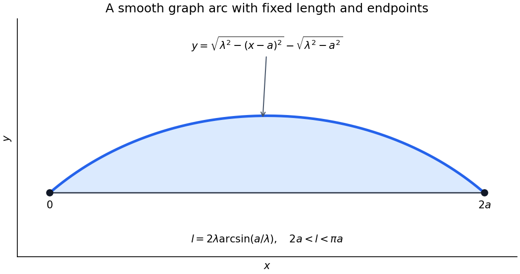
For the upper function graph, the vertical cross-section of the enclosed region has length $y(x)$, so its area is $J[y]={\int }_0^{2a}y(x)dx$. A maximizing nonnegative arch therefore uses $F=y$ and $G=\sqrt{1+y^{\prime 2}}$ in the normal Euler-Lagrange equation. It becomesIntegrating once gives $y^{\prime }/\sqrt{1+y^{\prime 2}}=(c-x)/\lambda$. The concave upper branch has $\lambda >0$ and integrates to $y=\sqrt{{\lambda }^2-(x-c{)}^2}+d$. The equal zero endpoint heights force $c=a$ and $d=-\sqrt{{\lambda }^2-a^2}$. HenceIt is a circular arc. To find its parameter, substitute into the length integral: $\sqrt{1+y^{\prime 2}}=\lambda /\sqrt{{\lambda }^2-(x-a{)}^2}$, givingThis scalar equation determines $\lambda$ numerically when needed; no explicit solution is required.

The arch is a global maximum in its smooth function graph regime. For $\lambda >0$, the integrand $y-\lambda \sqrt{1+y^{\prime 2}}$ is concave and strictly concave in its slope. Its supporting-tangent inequality, integrated against any competing function graph with the same endpoint values, has first-order term zero by the Euler-Lagrange equation. Thus $J[y]-\lambda I[y]\le J[y_{\ast }]-\lambda I[y_{\ast }]$. On the fixed-length class this is $J[y]\le J[y_{\ast }]$; strict slope concavity also gives uniqueness.

The source leaves the length range implicit. A twice continuously differentiable function graph of this form needs $\lambda >a$, giving $2a<l<\pi a$. At $l=2a$ the straight function graph is the degenerate solution. The semicircle limit $l=\pi a$ has vertical endpoint tangents and is outside that smooth function graph class. For $l>\pi a$, no arc in the claimed smooth function graph family exists, so the stated formula cannot describe a twice continuously differentiable maximizing function graph under those unrestricted data. Allowing overhanging curves changes the admissible class.

Write $K[y]={\int }_a^{b}G(x,y,y^{\prime })dx$. At a regular constrained extremal, the first variation of $K$ is not identically zero. Choose a variation $\zeta$ for which $\delta K[\zeta ]\ne 0$; the implicit function theorem supplies a correction in the $\zeta$ direction to each other variation so that $K$ remains one. Stationarity of $J$ on these corrected variations implies $\delta J=\lambda \delta K$ for one scalar $\lambda$.

Put $L=F-\lambda G$. Integration by parts gives, for an arbitrary twice continuously differentiable variation $\eta$,Taking variations with zero endpoint values and using the stated fundamental lemma of the calculus of variations gives the Euler-Lagrange equation. The remaining endpoint values are free and independent, giving the natural boundary conditions:If the constraint is not regular, the general multiplier statement permits an abnormal pair ${\lambda }_{0}F-{\lambda }_{1}G$ with ${\lambda }_0=0$; the source's general normal-form derivation implicitly excludes that case. In its quadratic example, regularity follows automatically from normalization: $\delta K[y]=2\int w{y}^2=2$.

For that example $L=p{y}^{\prime 2}-q{y}^2-\lambda w{y}^2$, so the equation and endpoint conditions reduce toMultiply the equation by $y$ and integrate. The boundary term $[p{y}^{\prime }y{]}_a^b$ vanishes, givingThe last integral equals one, so $\lambda =J[y]$, the functional value at the constrained extremal.

Finally multiply the equation for $y_1$ by $y_2$ and the equation for $y_2$ by $y_1$, then subtract and integrate. The derivative terms give only the vanishing boundary term $[p(y_2{y}_1^{\prime }-y_1{y}_2^{\prime }){]}_a^b$, while the $q$ terms cancel. Therefore $({\lambda }_1-{\lambda }_2){\int }_a^{b}w{y}_1{y}_{2}dx=0$. For distinct multipliers this proves

Discard the constant factor $2\pi$ when forming the Euler-Lagrange equation. For $F=y\sqrt{1+y^{\prime 2}}$ it becomesThe Beltrami identity, since $F$ has no explicit $x$ dependence, gives $F-y^{\prime }{F}_{y^{\prime }}=y/\sqrt{1+y^{\prime 2}}=C>0$. Combining with the differential equation yields $y^{\prime \prime }=y/C^2$. Its exponential solution has coefficients whose product is $C^2/4$, by $y^{\prime 2}=y^2/C^2-1$. Positivity therefore puts it in the formIts constants must satisfy $y_1=C\cosh ((x_1-K)/C)$ and $y_2=C\cosh ((x_2-K)/C)$. Depending on the endpoint data, these equations may have no solution or more than one. A constant function can satisfy a formal first-integral equation but fails the full Euler-Lagrange equation; it is not an extra extremal.