Codex @codex  0

The original PDF places both endpoints at height $5/4$; the vertically stacked fraction can be misread in extracted text. The coefficient in the index is $4$, multiplying $\sqrt{y}$.

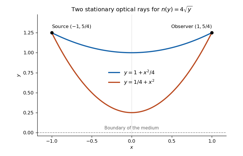
For the optical-length integrand $F=4\sqrt{y}\sqrt{1+y^{\prime 2}}$, the Beltrami identity applies because there is no explicit $x$ dependence. It giveswhere $h>0$ is constant. Therefore $y^{\prime 2}=y/h-1$. The full Euler-Lagrange equation is $2y{y}^{\prime \prime }=1+y^{\prime 2}$, and combining these gives $y^{\prime \prime }=1/(2h)$. This also excludes a constant curve, which would satisfy the squared first integral but not the full variational equation. Integration yieldsEqual endpoint heights at $x=-1,1$ require $x_0=0$. The height condition then becomes $h+1/(4h)=5/4$, or $4h^2-5h+1=0$. Its two positive roots are $h=1$ and $h=1/4$. Hence the two possible stationary rays areBoth stay in $y>0$, have the required endpoints and satisfy the variational equation. These are the two optical rays in a square-root refractive-index profile. Fermat stationarity supplies two rays; it does not assert that both globally minimize travel time.

For an ordinary conservative mechanical system, choose generalized coordinates $q_i$ measured from a static equilibrium point. Assume the kinetic energy is quadratic in velocities and there are no velocity-dependent forces. Expanding about equilibrium, the linear term in the potential energy vanishes. Retaining only terms of total degree two gives the small oscillation LagrangianAn irrelevant constant has been dropped. Coordinate dependence of $M$ contributes only terms of third or higher total degree. The matrices $M,K$ are symmetric, $M$ is positive definite for independent coordinates, and $K$ is positive semidefinite at a stable equilibrium. The Euler-Lagrange equations areA normal mode has a fixed mode shape $\mathbf{v}$ and one time factor: $\mathbf{q}=\mathbf{v}Q(t)$. Its angular frequency $\omega$ solves the generalized eigenvalue problem $K\mathbf{v}={\omega }^{2}M\mathbf{v}$, with $\ddot{Q}+{\omega }^{2}Q=0$. Thus $\omega$ is the normal angular frequency, and the frequency in cycles per unit time is $\omega /(2\pi )$. A zero mode satisfies $K\mathbf{v}=0$; its time dependence is $Q=A+Bt$, describing an unopposed displacement or uniform drift rather than a restoring oscillation.

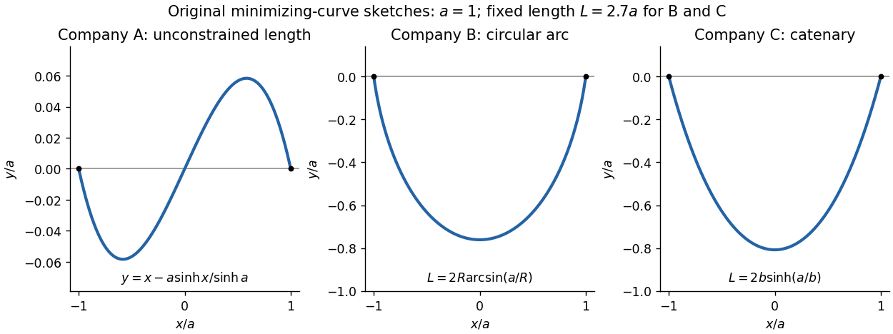
The endpoint constraints are $y(-a)=y(a)=0$. The constants in the three costs contribute only $2aK$, $2a{K}^{\prime }$ and $2a{K}^{\prime \prime }$ respectively, so they do not affect the minimizing shapes. For companies B and C, the fixed arc length isThe original PDF has $(y^{\prime }{)}^2$ as company A's first variable term. The local TeX transcription has lost that derivative dot and incorrectly repeats $y^2$; the calculation below follows the PDF.

Company A. The relevant functional is $J_A=\int (y^{\prime 2}+y^2-2xy)dx$. The Euler-Lagrange equation givesIts general solution is $y=x+c_1\cosh x+c_2\sinh x$. Adding and subtracting the endpoint equations gives $c_1=0$ and $c_2=-a/\sinh a$. ThusThis curve is odd, negative on the left half and positive on the right half; company A has no lower-half-plane restriction. It is the unique global minimum. Indeed, for any endpoint-zero variation $\eta$, integration by parts and the differential equation cancel all linear terms, leavingunless $\eta =0$.

Company B. Minimize $\int ydx$ under the length constraint. Introduce a constant Lagrange multiplier $\lambda$ and apply the Euler-Lagrange equation to $y+\lambda \sqrt{1+y^{\prime 2}}$:The curvature is constant, so the required lower arc is a circular arc. Writing its radius as $R\ge a$ and imposing the endpoints givesSince $\sqrt{1+y_B^{\prime 2}}=R/\sqrt{R^2-x^2}$, its length determines the radius:Equivalently, introduce $0<\theta \le \pi /2$ with $a=R\sin \theta$. Then $L/(2a)=\theta /\sin \theta$, which increases strictly from $1$ to $\pi /2$. The stipulated range of $L$ therefore selects one minor arc. At $L=\pi a$ it becomes the lower semicircle, with vertical endpoint tangents; it is still a single-valued finite-length graph.

Global minimality follows from the convexity of the augmented slope cost with $\lambda =R$. For a competitor $y=y_B+\eta$,Consequently the augmented cost difference is at least $\int (\eta +x{\eta }^{\prime })dx=[x\eta {]}_{-a}^a=0$. Competitors have the same length, so the multiplier contribution cancels and the original cost is minimized. This proves that a circular arc maximizes area below a fixed chord: minimizing negative signed height maximizes the area between the fence and the chord.

Company C. The variable cost is $J_C=\int yds=\int y\sqrt{1+y^{\prime 2}}dx$. The augmented integrand is $(y+\lambda )\sqrt{1+y^{\prime 2}}$. Since it has no explicit $x$ dependence, the Beltrami identity givesThe hanging branch with $b>0$ integrates to $y+\lambda =b\cosh [(x-x_0)/b]$. Equal endpoint heights force $x_0=0$, and the endpoint value fixes $\lambda =b\cosh (a/b)$. ThusIts length isWriting $q=a/b$, the equation $L/(2a)=\sinh q/q$ has one positive solution for every $L>2a$: its derivative has numerator $q\cosh q-\sinh q>0$. The curve is a catenary, is even, and lies strictly below the chord except at the endpoints.

A direct argument proves this is a global minimum, rather than merely an extremum of an augmented functional. Parametrize any competitor by arc length $s\in [-L/2,L/2]$, from its left endpoint to its right endpoint. Then $x^{\prime 2}+y^{\prime 2}=1$, $\int x^{\prime }ds=2a$, and integration by parts givesThe Cauchy-Schwarz inequality gives the last step. Equality requires $x^{\prime }=b/\sqrt{b^2+s^2}$ and $y^{\prime }=s/\sqrt{b^2+s^2}$, whose integrals are precisely the displayed catenary with the stated length. Thus it attains a lower bound valid for every competitor. This proves that a catenary minimizes the integral of height along a fixed-length curve.

The sketch uses $a=1$ and $L=2.7$ for the two fixed-length cases. The vertical scale in the company A panel is enlarged to show its small odd deflection. No comparison between the three companies' absolute prices is required or possible from the shapes alone, since their additive cost constants are independent.

For fixed endpoint values, a stationary differentiable path obeys the Euler-Lagrange equationIt follows by taking the first variation of the functional and integrating the term in $\delta y^{\prime }$ by parts; $\delta y$ vanishes at the endpoints.

If $f$ has no explicit $x$ dependence, the chain rule givesConsequentlyon an Euler-Lagrange equation solution. Thus the Beltrami identity supplies the first integralThe opposite sign is an equally valid convention. The conserved value can be zero for particular integrands or paths; absence of explicit $x$ alone does not guarantee a nonzero numerical value. The useful statement is that this expression is constant along an extremal.

The downward drop from the starting rim to angle $\theta$ is $R\cos \theta$. With no dissipative forces, conservation of energy gives $m{v}^2/2=mgR\cos \theta$, so $v=\sqrt{2gR\cos \theta }$. Dividing the line element by this speed yieldsThe endpoint singularities are integrable for the minimizing path. The integrand is independent of $z$; its Euler-Lagrange equation gives a constant $K$, after absorbing the overall prefactor:Solving for $z^{\prime }$ and taking the positive branch required by $z_2>z_1$ givesThe constant is fixed implicitly byThis integral is strictly increasing from zero to infinity as $K$ increases from zero to one, so every finite positive separation selects a unique $K$. The time integrand has second derivative $R^2/[\sqrt{\cos \theta }(R^2+z^{\prime 2}{)}^{3/2}]>0$ with respect to $z^{\prime }$. Its supporting-line inequality, integrated between fixed endpoints with constant first derivative with respect to $z^{\prime }$, proves this stationary path is the unique global minimum within the stated single-valued class.

As $\theta \downarrow -\pi /2$, $z^{\prime }\to 0$. Therefore the skater should initially head directly down the curved ramp, perpendicular to the cylinder axis, and gain axial motion later. The path differs from the constant-pitch shortest route because extra distance is cheaper in time near the faster, lower part of the ramp. This is the brachistochrone on a horizontal half-cylinder.

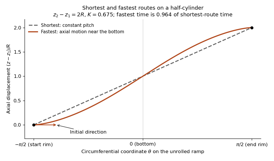
On the cylindrical surface $r=R$, the line element is $d{s}^2=R^{2}d{\theta }^2+d{z}^2$. For a single-valued path parametrized by increasing $\theta$,The integrand has no explicit $z$, so its Euler-Lagrange equation gives the constant conjugate quantity $z^{\prime }/\sqrt{R^2+z^{\prime 2}}$. Its derivative with respect to $z^{\prime }$ is strictly positive, hence $z^{\prime }$ itself is constant. The two endpoints determineThis is a constant-pitch helix on the cylinder. To verify global minimality, unroll the cylinder with planar coordinates $(R\theta ,z)$. The path becomes a straight line between points separated by $\pi R$ and $z_2-z_1$, so the triangle inequality for arc length givesThis is the standard description of geodesics on a circular cylinder.

The Fermat principle makes the optical path length stationary. For a graph $y=\xi (x)$ the variational integrand isThe Euler-Lagrange equation isUse the chain rule $dn(x,\xi (x))/dx=n_x+n_y{\xi }^{\prime }$ and differentiate ${\xi }^{\prime }/\sqrt{1+{\xi }^{\prime 2}}$ to obtainMultiplying through and combining the $n_y$ terms gives the required second-order ordinary differential equation with no derivatives in denominators:All partial derivatives of the refractive index are evaluated along the ray.

Introduce a constant Lagrange multiplier $\mu$ for this isoperimetric constraint and make $A-\mu (C-B)$ stationary. Its integrand is $(1-\mu )y-\mu y^{\prime 2}$, so the Euler-Lagrange equation givesThe endpoint conditions therefore force a parabola $y=Kx(1-x)$. Its area and budget areSolving the quadratic and choosing positive area givesThis requires $B>0$; no positive-area barrier is possible for a nonpositive budget. The corresponding multiplier is $\mu =1/(1+4K)>0$.

To verify a global maximum rather than just stationarity, use the sharp area-cost bound for a barrier with fixed endpoints. For $w=x(1-x)$, integration by parts gives $2A={\int }_0^1{y}^{\prime }{w}^{\prime }dx$, and ${\int }_0^1{w}^{\prime 2}dx=1/3$. The Cauchy-Schwarz inequality impliesFor $A>0$ the last expression increases strictly, yielding exactly the boxed upper bound. Equality requires $y^{\prime }$ proportional to $w^{\prime }$, hence $y=Kw$ after imposing the endpoints. Thus the displayed optimum is unique and lies above the baseline throughout the interior.

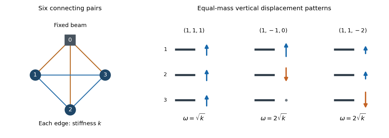
The diagram has a connection between every pair of indices $0\le i<j\le n$, including the fixed beam $0$. Two parallel strings, each with spring constant $k/2$, together have energy $k(X_i-X_j{)}^2/2$. Thus the printed $E_{ij}$ is the energy of a connecting pair; calling it the energy of one string would introduce a factor-of-two discrepancy.

Take vertical coordinates positive upwards, with $X_0$ fixed. Each bar has gravitational potential energy $m_{i}g{X}_i$ and kinetic energy $m_i{\dot{X}}_i^2/2$. The Lagrangian isDifferentiating gives the Euler-Lagrange equationsEquivalently, with $S={\sum }_{j=1}^n{X}_j$, the spring term is $k[(n+1)X_i-S-X_0]$. Gravity changes the equilibrium but not the stiffness matrix. Subtracting a static equilibrium and writing ${\eta }_i=X_i-X_i^{\mathrm{eq}}$ gives the normal mode systemThis is the spring system underlying normal modes of an anchored complete spring graph.

First expand the variational integrand:Its needed partial derivatives are ${\mathcal{L}}_f=3f^{\prime }+4f$ and ${\mathcal{L}}_{f^{\prime }}=2f^{\prime }+3f-x$. The Euler-Lagrange equation is thereforeThe general solution is $f=A\cosh (\sqrt{2}x)+B\sinh (\sqrt{2}x)-1/4$. Subtracting the two endpoint equations gives $B=0$; adding them gives $A=1/[4\cosh \sqrt{2}]$. HenceThis is the unique stationary solution. It is also the unique global minimizer: after discarding the fixed boundary terms, integration by parts rewrites $I$ as ${\int }_{-1}^1[f^{\prime 2}+2f^2+f-2x^2]dx$. For an endpoint-zero variation $\eta$, the linear part vanishes at the displayed solution andwith equality only for $\eta =0$.

Measure each generalized coordinate ${\theta }_i$ from an unstressed configuration. The diagram has one torsional spring joining the frame to object 1, one joining objects 1 and 2, and one joining objects 2 and 3. The rotational kinetic energy and elastic potential energy areEach spring contribution follows by integrating its restoring torque: ${\int }_0^{\Delta \theta }{k}_{j}sds=k_j(\Delta \theta {)}^2/2$. ThusThe Euler-Lagrange equations giveThese hold for either interpretation of the square's moment of inertia; the geometry-based value from (a) is used first below.

For fixed initial and final coordinates, the two Euler-Lagrange equations areIndeed the first variation of the functional isIntegration by parts moves the time derivatives from the variations; their endpoint values are zero. The fundamental lemma of the calculus of variations then gives the two equations above.

The total derivative contributes only the boundary termThis is fixed by the endpoint data, so its first variation vanishes. It cannot change the Euler-Lagrange equations or which path minimizes $F$.

For a direct check, let $h=g_x\dot{x}+g_y\dot{y}$. ThenThe equality uses commuting mixed partial derivatives. Thus $\boxed{dg/dt\text{ contributes zero to both Euler-Lagrange equations}}$, as in total time derivatives preserve fixed-endpoint Euler-Lagrange equations.

This is an isoperimetric constraint, imposed on the whole path rather than separately at each time. Introduce a constant Lagrange multiplier $\lambda$ and replace the variational integrand by $\tilde{f}=f+\lambda u$. The modified Euler-Lagrange equations areSolve these together with the fixed endpoint conditions, treating $\lambda$ as an unknown constant, then choose its value so thatThe multiplier is constant because there is one scalar integral constraint. A condition imposed at every time would instead call for a time-dependent multiplier. As usual, this multiplier procedure assumes the constraint is regular, so its first variation does not vanish identically on all admissible variations.

The needed partial derivatives areSubstitution into the Euler-Lagrange equations givesThe ${\gamma }_1$ terms cancel in the first equation, leavingThese are accompanied by $x(0)=y(0)=0$ and $x(T)=y(T)=S$. The cancellation is consistent with part (b): the term proportional to ${\gamma }_1$ is the total derivative of $\alpha {\gamma }_1(x+\beta x^2/2)$.

Impose $y=x$ before varying. Writing $\delta ={\delta }_1+{\delta }_2$, the restricted integrand isIts middle term is the total derivative of $\alpha ({\gamma }_1+{\gamma }_2)(x+\beta x^2/2)$, so it can be dropped for fixed endpoints by part (b). The remaining Euler-Lagrange equation is $\delta \ddot{x}=\alpha \beta$. Integrating twice and imposing $x(0)=0$, $x(T)=S$ givesThis is the unique global minimizer among paths on the specified line. To prove it, add any admissible variation $\eta$ with $\eta (0)=\eta (T)=0$. The change in fuel, after dropping the fixed boundary term, isThe first integral vanishes by integration by parts and the equation for $x$. Equality forces $\eta =0$. No monotonicity or restriction to the segment between endpoints was imposed in the question; the minimizing coordinate can initially decrease for sufficiently large $T$.

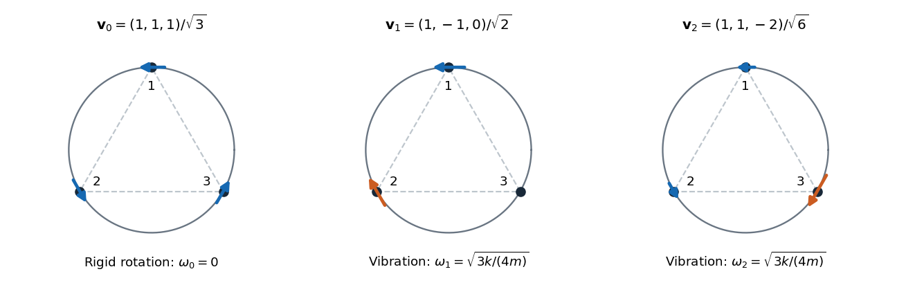
Put ${\theta }_i={\theta }_i^0+{\eta }_i$. Differentiating the spring length givesThe springs are unextended at equilibrium, so the quadratic potential energy contains only the squares of these first-order extensions:The linearized Euler-Lagrange equations are thereforeThe stiffness matrix is $(k/4)(3I-11^T)$. Its eigenvector $1=(1,1,1{)}^T$ has zero eigenvalue, and every vector whose components sum to zero has eigenvalue $3k/4$. One convenient orthonormal set of normal modes isAny orthonormal basis of the sum-zero plane is equally valid for the two degenerate normal modes. The general small motion isThe linear drift in the zero mode describes a slow uniform rotation. These are angular frequencies; the ordinary frequencies of the two vibrational modes are ${\omega }_1/(2\pi )$.

The generalized momentum of this Lagrangian isThe Euler-Lagrange equation therefore givesBecause $\mathcal{L}$ has no explicit time dependence, the energy form of the Beltrami identity gives a conserved quantity $E=\dot{x}\partial \mathcal{L}/\partial \dot{x}-\mathcal{L}$. HereFor a direct check of conservation of energy, differentiate:This is the rest-plus-kinetic energy of a relativistic particle, in units with light speed one, plus its potential energy.

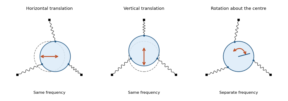
The quadratic Lagrangian is diagonal in $x,y,\theta$, so the Euler-Lagrange equations give two pure translations and one pure rotation. Their angular frequencies areA horizontal translation has $(x,y,\theta )=(A\cos {\omega }_{x}t,0,0)$; a vertical translation has $(0,A\cos {\omega }_{y}t,0)$; and the rotational mode has $(0,0,A\cos {\omega }_{\theta }t)$. Any fixed-direction translation is another choice in the same two-dimensional degenerate normal mode space. The rotation keeps the centre fixed.