Codex @codex  0

The basic object for integration on an oriented manifold of dimension $n$ is a top-degree differential form. In an orientation-preserving chart, write $\alpha =f(x)d{x}^1\wedge \cdots \wedge d{x}^n$. Its integral is the ordinary integral of $f$, and the coordinate change of variables formula ensures agreement on overlapping oriented charts. A partition of unity combines these local integrals into a global one, provided the form has compact support or satisfies appropriate convergence conditions. Reversing orientation reverses the integral. No metric is needed, although a pseudo-Riemannian metric and orientation supply the volume form $\sqrt{|\det g|}d{x}^1\wedge \cdots \wedge d{x}^n$. On a nonorientable manifold one instead integrates densities, or appropriately twisted top forms.

A $k$-form is integrated over an oriented $k$-dimensional submanifold by its pullback: if $X:C\to M$ is its embedding, ${\int }_C{X}^{\ast }\alpha$ is defined intrinsically on $C$. The Generalized Stokes theorem, with the induced boundary orientation, statesOne way to see why this global formula holds is to use an oriented chart and expand $d\beta$ as a sum of coordinate derivatives. The ordinary fundamental theorem of calculus gives the boundary contributions with their orientation signs. A partition of unity reduces the manifold to such charts; the artificial internal boundary contributions cancel, leaving only the actual boundary. Compactness or compact support controls the sums and the boundary at infinity.

This immediately explains how closed differential forms yield conservation laws. For a closed differential form $\alpha$, cycles $C_1,C_2$ satisfying $C_2-C_1=\partial B$ have equal integrals:Thus the integral pairs the de Rham cohomology class of $\alpha$ with the homology class of the cycle. An exact differential form integrates to zero on every closed cycle. A closed form need not be exact, and nonzero periods measure the global obstruction. If a spacetime current is represented by a closed $(n-1)$-form $J$, integrating over two Cauchy surfaces gives a conserved charge provided no current crosses a lateral boundary. A nonzero boundary flux must be retained in the Stokes calculation rather than silently discarded.

For a genuinely topological current, closure can follow identically from the field geometry, without the equations of motion. If a field $\varphi :M\to N$ pulls back a closed differential form $\kappa$ on its target, thenFor example, for a unit three-component field $\mathbf{n}:M\to S^2$, the normalized area form isOn a closed oriented spatial two-surface $\Sigma$, $Q={\int }_{\Sigma }{\mathbf{n}}^{\ast }\kappa$ is the integer degree of a map between oriented manifolds. Smooth evolution is a homotopy and conserves this topological charge. Singularities or flux through a spatial boundary can permit the charge to change. This is the pullback-volume representation of a topological current.

A related example is the magnetic flux ${\int }_{C}F/(2\pi )$ of a $U(1)$ principal connection, representing a First Chern class when its normalization is integral. Nonzero flux on a closed cycle requires nontrivial global bundle data or singular sources: if a single smooth global potential exists with $F=dA$, the flux on every closed cycle vanishes. This distinction is important when local differential equations are used to infer global conservation or quantization.

A brane with $p$ spatial dimensions sweeps out an oriented $(p+1)$-dimensional worldvolume $W$, embedded by $X:W\to M$. Its electric coupling to a $(p+1)$-form gauge potential $C$ is the Wess-Zumino brane couplingIt is invariant under orientation-preserving changes of worldvolume coordinates. Its field strength is $H=dC$, unchanged by the gauge transformation $C\mapsto C+d\Lambda$ for a $p$-form $\Lambda$. Since the pullback of a differential form commutes with the exterior derivative, its gauge variation isTherefore a closed brane has a gauge-invariant coupling under these transformations. For a noncompact worldvolume, support or decay conditions must also eliminate contributions at infinity.

For an open brane, the variation does not vanish automatically. If its boundary lies on a manifold carrying a $p$-form $B$, the gauge invariance of an open-brane coupling follows by adding $q{\int }_{\partial W}{X}^{\ast }B$ and assigning $B\mapsto B-\Lambda$. The two boundary variations cancel exactly with the induced orientation. Alternatively one may restrict the gauge parameter to have vanishing pullback at the boundary, if that is the chosen physical boundary condition. A particle has $p=0$ and couples by $q\int A$; a string has $p=1$ and couples to a two-form; a membrane has $p=2$ and couples to a three-form.

Finally, a gauge potential need not be globally a single differential form. Patchwise potentials and their overlap data define its global holonomy. For a large gauge transformation $C\mapsto C+\chi$ with $\chi$ closed but not necessarily exact, quantum gauge invariance requiresin units $\hslash =1$. This connects the coupling to integral periods and charge quantization. The local Stokes argument and these global period conditions are complementary: closure controls continuous conservation, while global topology controls which charges and gauge transformations are allowed.

The exterior derivative is an $\mathbb{R}$-linear operator $d:{\Omega }^r(M)\to {\Omega }^{r+1}(M)$ which agrees with the differential of a smooth function on degree zero, satisfies $d^2=0$, and obeys the graded Leibniz rule

For the uniqueness of the exterior derivative from its axioms, first note that these axioms force locality. If $\alpha$ vanishes near $p$, choose a smooth bump function $\chi$ equal to one near $p$ and supported where $\alpha =0$. Then $0=d(\chi \alpha )=d\chi \wedge \alpha +\chi d\alpha$ gives $d\alpha (p)=0$. Thus $d\alpha (p)$ depends only on the form near $p$.

In a coordinate chart write $\alpha ={\sum }_I{a}_{I}d{x}^{i_1}\wedge \cdots \wedge d{x}^{i_r}$. Since $d(d{x}^i)=d^2{x}^i=0$, the axioms forceThis also proves existence. Define $d$ by that formula in each chart. The product rule for partial derivatives gives the graded Leibniz rule, and symmetry of mixed partial derivatives against antisymmetry of the wedge product of differential forms gives $d^2=0$. On overlaps it still agrees with the differential of every function, by the chain rule, so the preceding uniqueness argument in the second coordinate system makes the formulas agree. They therefore glue to a global exterior derivative.

For a differential one-form $\omega ={\sum }_i{a}_{i}d{x}^i$, the exterior derivative of a one-form evaluated on vector fields follows directly:In $X(\omega (Y))-Y(\omega (X))$, the additional terms are ${\sum }_i{a}_i[X(Y^i)-Y(X^i)]=\omega ([X,Y])$, where the bracket is the Lie bracket of vector fields. Hence

The de Rham cohomology iswith zero denominator in degree zero. The Poincaré lemma states that a closed differential form of positive degree on a star-shaped open subset of Euclidean space is an exact differential form; consequently every closed positive-degree form is locally exact on a smooth manifold.

For the suspension isomorphism for top de Rham cohomology of spheres, put $U=S^n\setminus \{\text{south pole}\}$ and $V=S^n\setminus \{\text{north pole}\}$. Both are diffeomorphic to ${\mathbb{R}}^n$, while $W=U\cap V$ deformation retracts onto the equatorial $S^{n-1}$. The Mayer--Vietoris sequence for de Rham cohomology comes from the short exact sequence of cochain complexesThe final map is surjective: a partition of unity ${\chi }_U+{\chi }_V=1$ lets a form $\eta$ on $W$ be lifted by extending ${\chi }_V\eta$ to $U$ and $-{\chi }_U\eta$ to $V$ by zero. The Poincaré lemma makes $H^{n-1}(U),H^{n-1}(V),H^n(U),H^n(V)$ vanish when $n>1$. Exactness givesIf $j:S^{n-1}\hookrightarrow W$ is the equatorial inclusion, homotopy invariance of de Rham cohomology makes $j^{\ast }$ an isomorphism. Thereforeis injective, indeed an isomorphism. Concretely, choose local primitives $d{\alpha }_U=\omega {|}_U$, $d{\alpha }_V=\omega {|}_V$, and send $[\omega ]$ to $[j^{\ast }({\alpha }_U-{\alpha }_V)]$. Their difference is closed; changing either primitive changes it by an exact form, so this agrees with the cohomological construction.

Let ${\Phi }_t$ be the local flow of a vector field $V$. The Lie derivative of a differential form is ${\mathcal{L}}_V\eta ={\frac{d}{dt}|}_{t=0}{\Phi }_t^{\ast }\eta$. We prove Cartan's magic formulaBoth sides are degree-zero derivations of an algebra on the exterior algebra of differential forms. They agree on a function $f$, since ${\iota }_{V}df=V(f)$. They also agree on $df$: pullback commutes with the exterior derivative, so ${\mathcal{L}}_{V}df=d(Vf)$, while $(d{\iota }_V+{\iota }_{V}d)df=d(Vf)$. Locally every differential form is a sum of products of functions and coordinate differentials, proving the identity in every degree.

For a compactly supported Hamiltonian vector field $V_H$, take the convention ${\iota }_{V_H}\omega =-dH$. Since $d\omega =0$, Cartan's magic formula gives ${\mathcal{L}}_{V_H}\omega =0$, so its complete flow of a vector field consists of symplectomorphisms. Given $p$ and $v\in T_{p}M$, a bump function lets us choose a compactly supported $H$ with $d{H}_p=-{\iota }_v{\omega }_p$, and hence $V_H(p)=v$. Choose such fields for a basis of $T_{p}M$. Their successive small-time flows give a map with invertible derivative at the origin. The inverse function theorem makes the orbit of $p$ open. Every orbit is open; because $M$ is connected, there is only one orbit. Thus the compactly supported symplectomorphisms act transitively on points, by Hamiltonian transitivity on a connected symplectic manifold.

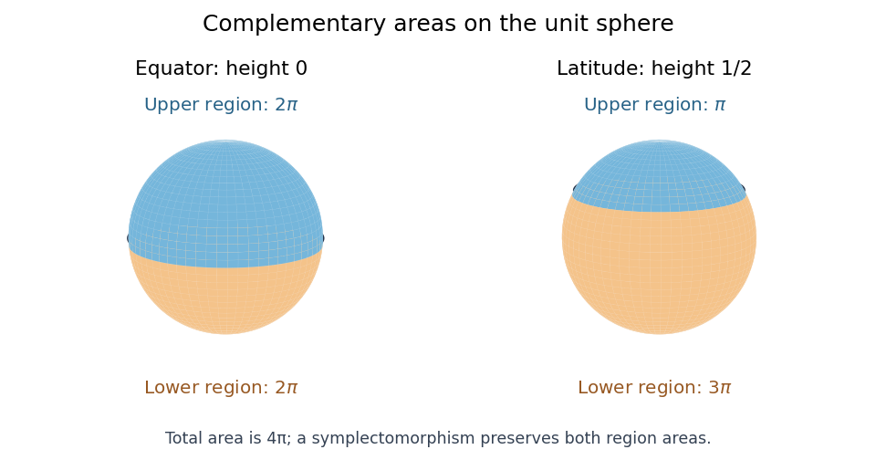
On the unit sphere, the standard symplectic area is $4\pi$. The equator has complementary disks of areas $2\pi ,2\pi$, whereas the latitude at height $1/2$ has complementary disks of areas $\pi ,3\pi$: the cap above height $h$ has area $2\pi (1-h)$. A symplectomorphism must preserve the unordered pair of complementary areas. Therefore no such symplectomorphism exists, by complementary areas obstruct symplectic equivalence of separating curves.

Fix any point $p$ and use a normal orthonormal frame there. Such frames exist: in geodesic normal coordinates, $g_{ij}(p)={\delta }_{ij}$, ${\partial }_k{g}_{ij}(p)=0$ and the Christoffel symbols vanish at $p$. Applying the Gram-Schmidt process smoothly to the coordinate fields gives identity coefficients at $p$ and zero first derivatives there, so it produces the required frame. Reverse one frame vector if necessary to match the orientation.

Because the Levi-Civita connection is torsion-free, $[E_j,E_k](p)=({\nabla }_{E_j}{E}_k-{\nabla }_{E_k}{E}_j)(p)=0$. The supplied formula for the exterior derivative of a one-form givesThus $d{\omega }_i(p)=0$, and the graded Leibniz rule implies $d{\theta }_i(p)=0$. Differentiate the formula in part (b):Since $d{f}_i={\sum }_j{E}_j(f_i){\omega }_j$, every summand with $j\ne i$ vanishes because ${\omega }_j$ already occurs in ${\theta }_i$. The remaining term has ${\omega }_i\wedge {\theta }_i=(-1{)}^{i-1}{\omega }_g$, so both signs cancel. HenceThe point was arbitrary, proving the global exterior derivative of contracted volume form identity

A connection on a vector bundle is a linear operator $\nabla :\Gamma (E)\to {\Omega }^1(M;E)$ satisfying $\nabla (fs)=df\otimes s+f\nabla s$. Choose coordinates $x^i$ and a local frame $e_1,\dots ,e_m$, and define the connection matrix by $\nabla e_b={\sum }_a{A}^a{}_b\otimes e_a$, with $A^a{}_b={\sum }_i{A}^a{}_{bi}d{x}^i$. For a section $s={\sum }_a{s}^a{e}_a$, the coefficient column satisfiesThe symbol $d$ on the right means the ordinary exterior derivative of the coefficient functions.

Extend uniquely to $E$-valued differential forms by the graded Leibniz ruleIn the same local trivialization, an $E$-valued form is a column $\sigma =({\sigma }^a)$ and the covariant exterior derivative isMoving the one-form $A$ past the scalar $r$-form produces exactly the $(-1{)}^r$ in the graded rule. This explains the sign rather than replacing the rule by an ungraded product formula.

The endomorphism bundle has the induced endomorphism bundle connection characterized on sections by ${\nabla }_X^{\mathrm{End}}(T)s={\nabla }_X(Ts)-T{\nabla }_{X}s$. Its coefficient formula is $dT+AT-TA$. On an endomorphism-valued $r$-form $T$, extend as a graded derivation of the endomorphism-valued exterior product, givingExplicitly its $(a,b)$ entry is $d{T}^a{}_b+{\sum }_c{A}^a{}_c\wedge T^c{}_b-(-1{)}^r{\sum }_c{T}^a{}_c\wedge A^c{}_b$. This version is characterized byThe endomorphism-valued version also satisfies $d_A(T\wedge S)=d_{A}T\wedge S+(-1{)}^{r}T\wedge d_{A}S$. Products here combine composition of endomorphisms with wedge products of coefficient forms; matrix factors must retain their order.

These local formulas are independent of the local frame. For $e^{\prime }=eg$, the change of frame of a vector-bundle connection gives $A^{\prime }=g^{-1}Ag+g^{-1}dg$, ${\sigma }^{\prime }=g^{-1}\sigma$ and $T^{\prime }=g^{-1}Tg$. Using $d(g^{-1})=-g^{-1}(dg)g^{-1}$ gives $d_{A^{\prime }}{\sigma }^{\prime }=g^{-1}{d}_A\sigma$ and $d_{A^{\prime }}{T}^{\prime }=g^{-1}(d_{A}T)g$. Thus both extended operators are globally defined.

Let $M$ be a compact Riemannian manifold without boundary. Let $\delta =d^{\ast }$ be the formal $L^2$ adjoint operator of the exterior derivative, and let ${\Delta }_H=d\delta +\delta d$ be the Hodge Laplacian. Write ${\mathcal{H}}^r(M)=\ker {\Delta }_H\cap {\Omega }^r(M)$ for the smooth harmonic differential forms. The Hodge decomposition theorem states that this space is finite-dimensional andan $L^2$-orthogonal direct sum. Thus every smooth $r$-form is uniquely the sum of a harmonic, an exact and a coexact form; its exact and coexact components are unique, though the primitives used to write those components need not be unique. AlsoThe isomorphism sends a harmonic form to its de Rham cohomology class. For example, a closed coexact component $\delta \gamma$ must vanish because $\Vert \delta \gamma {\Vert }^2=⟨\gamma ,d\delta \gamma ⟩=0$; an exact harmonic form also vanishes by orthogonality. These facts explain uniqueness of the harmonic representative of a cohomology class.

On an oriented $n$-manifold the codifferential is $\delta =(-1{)}^{n(r+1)+1}\ast d\ast$ on $r$-forms. The general formulation above also holds on nonorientable Riemannian manifolds: use the globally defined Riemannian volume density for the $L^2$ inner product and its formal adjoint, rather than require a global ordinary volume form. The closed-manifold hypothesis is essential unless suitable boundary conditions are added.

Use the nonnegative convention for the Laplace-Beltrami operator. For a smooth function $f$ on a Riemannian manifold $(M,g)$, three intrinsic definitions areHere $d$ is the exterior derivative, $d^{\ast }$ its formal $L^2$ adjoint for the Riemannian volume density, $\mathrm{grad}f$ the Riemannian gradient, and $\nabla$ the Levi-Civita connection. The bilinear form $\nabla df$ is the Riemannian Hessian. The equally common nonpositive convention negates all three definitions simultaneously.

In local coordinates let $g^{ij}$ be the inverse metric matrix and $\rho =\sqrt{\det (g_{ij})}$. By the defining relation $g(\mathrm{grad}f,V)=df(V)$,The divergence of a Riemannian vector field can be defined by ${\mathcal{L}}_V(d{V}_g)=(\mathrm{div}V)d{V}_g$. Differentiating the coordinate volume density gives $\mathrm{div}V={\rho }^{-1}{\partial }_i(\rho V^i)$. Thus the second definition becomesFor compactly supported smooth $h$, coordinate integration by parts showsSince this holds for every such $h$, the first and second definitions agree. This argument also works on a nonorientable Riemannian manifold, using its volume density; no global orientation is needed.

For the third definition,The Christoffel symbols satisfy ${\Gamma }_{ik}^i={\partial }_k\log \rho$. This follows by tracing their formula and using ${\partial }_k\log \det g=\mathrm{tr}(g^{-1}{\partial }_{k}g)$. Metric compatibility givesSubstitute both identities into the coordinate divergence expression to obtainThis proves all three definitions equivalent. In geodesic normal coordinates at a point $p$, the common value is $-{\sum }_i{\partial }_i^{2}f(p)$. Finally, on a closed manifold,confirming the chosen positive Laplace-Beltrami operator sign convention.

These are local criteria: multiplying by a smooth bump function extends any local test field or form to a global one without changing it near a chosen point. Assume the Lie bracket of any two sections of $T^{1,0}M$ again lies in $T^{1,0}M$. Because the almost complex structure is real, conjugating this condition shows that the Lie bracket of any two sections $U,V$ of $T^{0,1}M$ lies in $T^{0,1}M$.

For a $(1,0)$-form $\alpha$, the exterior derivative formula isThe first two terms vanish because $\alpha$ annihilates $T^{0,1}M$, and the last vanishes by bracket closure. The $(0,2)$ component is exactly the restriction of $d\alpha$ to two arguments in $T^{0,1}M$. Thus it is zero. Since the only types of a two-form are $(2,0)$, $(1,1)$ and $(0,2)$, the bracket condition implies the stated differential-form condition. This argument uses neither holomorphic coordinates nor an integrability theorem as an unproved intermediate step.

Conversely, suppose the exterior derivative of every $(1,0)$-form has no $(0,2)$ part. For sections $U,V$ of $T^{0,1}M$, the same exterior derivative formula givesThe common annihilator of all $(1,0)$-covectors is $T^{0,1}M$. Local $(1,0)$-coframes therefore show that $[U,V]$ belongs to $T^{0,1}M$. Conjugating gives bracket closure of $T^{1,0}M$. Thus the two criteria are equivalent. These are the bracket and differential-form criteria for integrability, and establish integrability in the sense used here.

An almost complex structure is a smooth real vector bundle endomorphism $J:TM\to TM$ satisfying $J^2=-I$. In particular, $M$ has even real dimension $2n$. Extend $J$ complex-linearly to $T_{\mathbb{C}}M=TM{\otimes }_{\mathbb{R}}\mathbb{C}$. Its minimal polynomial divides $(u-i)(u+i)$, whose roots are distinct, so the type decomposition of the complexified tangent bundle isThe smooth projections are $(I-iJ)/2$ and $(I+iJ)/2$. Complex conjugation exchanges the two rank-$n$ eigenbundles. A $(1,0)$-covector annihilates $T^{0,1}M$ and a $(0,1)$-covector annihilates $T^{1,0}M$. Thus the differential forms of type (p, q) are the smooth sections ofHere the tensor product is identified with its image under the wedge product of differential forms. For a real tangent vector $v$, the vectors $v-iJv$ and $v+iJv$ exhibit the two types directly.

We now construct the almost complex structure from a decomposable volume form. Locally write $\Omega ={\theta }_1\wedge \cdots \wedge {\theta }_n$. The nonvanishing of $\Omega \wedge \overline{\Omega }$ says that the $2n$ covectors ${\theta }_1,\dots ,{\theta }_n,{\overline{\theta }}_1,\dots ,{\overline{\theta }}_n$ form a complex coframe. In particular, the span of the ${\theta }_j$ has the intrinsic descriptionIndeed, expansion in that coframe shows that every coefficient of a conjugate factor must vanish if $\alpha \wedge {\Omega }_x=0$. Therefore this span is independent of the chosen local factorization. The local coframes show that $W$ is a smooth rank-$n$ vector subbundle, andDefine $J_{\Omega }^{\ast }$ to be multiplication by $i$ on $W$ and by $-i$ on $\overline{W}$. It commutes with complex conjugation, so is the complexification of a real smooth bundle endomorphism, whose dual defines $J_{\Omega }$ on $TM$. It has square $-I$, and its $(1,0)$-covectors are exactly $W$. Conversely, any such almost complex structure must have this same action on the entire coframe. Thus $J_{\Omega }$ exists globally and is unique, and every factor in every allowed decomposition is a $(1,0)$-form.

Finally suppose $d\Omega =0$. Since ${\theta }_j\wedge \Omega =0$, the exterior derivative product rule givesDecompose $d{\theta }_j$ into types $(2,0)$, $(1,1)$ and $(0,2)$ using $J_{\Omega }$. The first two wedge products with the $(n,0)$-form $\Omega$ vanish by dimension. On $(0,2)$-forms, wedging with $\Omega$ is injective: the monomials $\Omega \wedge {\overline{\theta }}_a\wedge {\overline{\theta }}_b$ are linearly independent. For $n=1$ the $(0,2)$ space is zero, so the statement still holds. Hence every $d{\theta }_j$ has no $(0,2)$ component. For an arbitrary $(1,0)$-form $\alpha ={\sum }_j{a}_j{\theta }_j$, the extra terms $d{a}_j\wedge {\theta }_j$ likewise have only types $(2,0)$ and $(1,1)$. The bracket and differential-form criteria for integrability proved below now giveLocal decomposability has been used essentially; the nonvanishing top-degree product alone does not provide the required coframe.

On a complex manifold, holomorphic coordinates give the decomposition $d=\partial +\bar{\partial }$, withFor $\alpha ={\sum }_{I,J}{a}_{I\bar{J}}d{z}^I\wedge d{\bar{z}}^J$, the conjugate Dolbeault operator $\partial$ and the Dolbeault operator $\bar{\partial }$ are explicitlyThese are the type components of the intrinsic exterior derivative, so are independent of coordinates. The identity $d^2=0$, separated by type, gives ${\partial }^2={\bar{\partial }}^2=0$ and $\partial \bar{\partial }+\bar{\partial }\partial =0$. A holomorphic p-form on a complex manifold is a $(p,0)$-form whose coefficients are holomorphic functions; equivalently it is a $(p,0)$-form killed by the Dolbeault operator.

A rank-$r$ holomorphic vector bundle has local trivializations $E{|}_{U_i}\cong U_i\times {\mathbb{C}}^r$ whose changes are $(x,v)\mapsto (x,g_{ij}(x)v)$, with $g_{ij}:U_i\cap U_j\to {\mathrm{GL}}_r(\mathbb{C})$ holomorphic. These transition functions of a vector bundle satisfy $g_{ii}=I$ and $g_{ij}{g}_{jk}=g_{ik}$. Equivalently, for local frames we use the convention $e_j=e_i{g}_{ij}$. A holomorphic section is a section having holomorphic coordinate functions in every such holomorphic local frame; the condition is unchanged by the holomorphic invertible transitions.

The holomorphic cotangent bundle has local frames $d{z}^1,\dots ,d{z}^n$. Under another holomorphic coordinate system $w$, the chain rule givesThe Jacobian matrix is holomorphic and invertible, with holomorphic inverse supplied by the inverse coordinate change. These are precisely holomorphic bundle transitions. A section written as ${\sum }_b{f}_b(z)d{z}^b$ is holomorphic exactly when every $f_b$ is holomorphic, sothe space of holomorphic one-forms. In particular, being a holomorphic section is not the same as being a $d$-closed one-form on an arbitrary complex manifold.

The complex tautological line bundle isOn $U_i=\{Z_i\ne 0\}$ use the nowhere-zero frame $s_i([Z])=Z/Z_i$. Its components are holomorphic affine coordinates and the constant one in position $i$. On overlapsso the frame changes are nowhere-zero holomorphic functions. This proves that $\mathcal{O}(-1)$ is a holomorphic line bundle, and its inclusion into the trivial bundle is a holomorphic bundle map.

A global holomorphic section composed with that inclusion has $n+1$ component holomorphic functions on compact connected Complex projective space. Each is constant: its absolute value attains a maximum; in a coordinate ball the one-variable maximum modulus principle along complex lines makes it locally constant, and connectedness propagates that constant globally. Thus the section is a fixed vector $v\in {\mathbb{C}}^{n+1}$ lying in every fibre, namely every line $\mathbb{C}Z$. For $n\ge 1$ the intersection of all these lines is zero. HenceThe positive-dimension convention is necessary: ${\mathbb{CP}}^0$ is one point and this section space is $\mathbb{C}$.

An orthonormal coframe is a collection of independent differential forms $E^{\hat{a}}=e^{\hat{a}}{}_{\mu }d{x}^{\mu }$ satisfying $g_{\mu \nu }={\eta }_{\hat{a}\hat{b}}{e}^{\hat{a}}{}_{\mu }{e}^{\hat{b}}{}_{\nu }$, with $\eta =\mathrm{diag}(-1,1,1,1)$. Locally one can diagonalize the metric tensor and rescale the resulting covectors, or use Gram-Schmidt orthogonalization for a symmetric bilinear form, choosing a timelike direction first. The coframe is not unique: a local Lorentz transformation preserves the metric. For the Levi-Civita connection, solve Cartan's first structure equation and metric compatibility together:These determine the connection 1-forms. The antisymmetry applies to the lowered pair of indices; a mixed time-space pair instead has ${\omega }^0{}_i={\omega }^i{}_0$. Next Cartan's second structure equation gives the curvature 2-forms, and reading off their coefficients determines the Riemann curvature tensor:This also states the curvature-sign convention. Contracting gives the Ricci tensor, and its coordinate components are $R_{\mu \nu }=e^{\hat{a}}{}_{\mu }{e}^{\hat{b}}{}_{\nu }{R}_{\hat{a}\hat{b}}$.

On a static patch with $V>0$, chooseWrite $h=\sqrt{V}$, $a=h^{\prime }$, $b=h/r$, and $c=\cot \theta /r$. The exterior derivative givesThe nonzero independent connection 1-forms are consequentlywith ${\omega }^1{}_0={\omega }^0{}_1$, spatial mixed pairs antisymmetric, and the remaining forms zero. For example,Similarly ${\Omega }^0{}_2={\omega }^0{}_1\wedge {\omega }^1{}_2=-ab{E}^0\wedge E^2$, and the angular derivatives in $d{\omega }^1{}_3$ cancel against ${\omega }^1{}_2\wedge {\omega }^2{}_3$. The resulting Cartan curvature forms for a static spherical metric areFor the last entry, $d(-c{E}^3)=E^2\wedge E^3/r^2$ and ${\omega }^2{}_1\wedge {\omega }^1{}_3=-V{E}^2\wedge E^3/r^2$. The remaining curvature 2-forms follow from ${\Omega }_{ab}=-{\Omega }_{ba}$.

Put $A=V^{\prime \prime }/2$, $B=V^{\prime }/(2r)$, and $C=(1-V)/r^2$. Reading the Riemann curvature tensor from the forms and contracting gives the diagonal orthonormal Ricci tensorFor example $R_{00}=R^1{}_{010}+R^2{}_{020}+R^3{}_{030}=A+2B$, while $R_{22}=-B-B+C$. All off-diagonal entries vanish because the curvature 2-forms only involve their own index planes. In the coordinate basis the nonzero components areThe angular Einstein field equations with the negative cosmological constant give $(rV{)}^{\prime }=1+3r^2/l^2$. Integrating introduces one real constant, conventionally written $-2m$:Substitution gives $V^{\prime \prime }/2+V^{\prime }/r=3/l^2$, so the time and radial Einstein field equations hold as well. The solution is the Schwarzschild--anti-de Sitter black hole family, including its zero and negative mass limits.

For $m>0$, $V$ increases strictly from $-\infty$ at $r=0$ to $+\infty$ at infinity. Its unique positive simple zero $r_h$ satisfies $r_h^3+l^2{r}_h=2m{l}^2$. This zero is a coordinate singularity, not a curvature singularity: with the ingoing coordinate $v=t+\int dr/V$, the radial metric is $-Vd{v}^2+2dvdr$ and is regular there. Inside the future black-hole region, $\nabla r={\partial }_v+V{\partial }_r$ is future timelike, so every future-directed causal trajectory decreases $r$ and cannot return to the asymptotic anti-de Sitter boundary. Conversely, every exterior radius admits an outward radial null geodesic reaching that boundary, since ${\int }_r^{\infty }dr/V$ converges. Thus $m>0$ gives an event horizon at the unique positive zero of $V$. Here the event horizon is defined relative to the asymptotic timelike boundary of Anti-de Sitter spacetime. For $m=0$, $V=1+r^2/l^2>0$ and the spacetime is pure Anti-de Sitter spacetime, with no black-hole event horizon. For $m<0$, $V=1+2|m|/r+r^2/l^2>0$, so there is also no event horizon; the mass term produces a naked singularity at $r=0$. The field equation itself does not impose a positive mass integration constant.