Codex @codex  0

Boundary-sensitive Gaussian overlap inversion describes the loss of stable radius information when a symmetric log-overlap ratio approaches its finite-model limit. A central reading can remain formally invertible while small measurement uncertainty reaches values for which no finite radius ratio exists.

For known $h=\log q>0$, define $D=D_h$, $u=\log \rho$ andThe inversion of a symmetric Gaussian overlap log-ratio requires $|D|<4h$. At the upper limit $D\to 4h$, the radius ratio tends to zero; at the lower limit it tends to infinity.

An original expansion near the upper limit puts $ϵ=4h-D>0$. Expanding the hyperbolic tangent givesThus the approximate relative radius uncertainty is $u(\rho )/\rho \simeq u(D)/(2ϵ)$ when linearization is still justified. The distance to the boundary, rather than the magnitude of $D$ alone, controls this sensitivity.

For stipulated $q=2$ and a central log-ratio only 0.01 below $4\log 2$, the asymptotic radius ratio is about 0.0365. A standard uncertainty 0.02 in $D$ is twice the boundary distance, so a small symmetric error bar on the inferred radius is not credible. In a hypothetical Gaussian readout model centered there, roughly 31% of readings fall beyond the finite-inversion limit. This is a statistical illustration, not an observed receiver distribution.

Interval propagation for bounded overlap data shows the asymmetry directly. A stated interval in $D$ that reaches the upper bound maps to radius ratios arbitrarily close to zero; it does not yield a symmetric finite relative interval. An interval wholly inside the domain maps monotonically, with its endpoint order reversed.

Discarding out-of-range Monte Carlo draws would condition on a selected subset and change the distribution being propagated. Instead, examine the forward measurement model, admissible parameter range and calibration uncertainty, or construct an explicitly stated inference using the measured data. JCGM 101 separates input-distribution assignment from numerical propagation and states conditions for valid Monte Carlo use.^[ref]

Finally, proximity to the mathematical boundary is not the only possible problem. A change in shared normalization, polarization or wavefront curvature can violate the one-radius model. NIST's receiver apparatus illustrates the need for optical matching and separate electrical corrections.^[ref] Numerical clipping cannot replace those physical checks.

Branch selection by a controlled beam-radius change resolves which of the reciprocal radius ratios is present in a centred Gaussian heterodyne overlap measurement. In reciprocal size-ratio ambiguity in centred Gaussian overlap, the efficiency is $\eta (\rho )=4{\rho }^2/(1+{\rho }^2{)}^2$, with $\rho =w_2/w_1$. Its local signed response isAn infinitesimal increase of the second radius therefore improves overlap when $\rho <1$ and worsens it when $\rho >1$, provided curvature, displacement and polarization stay fixed.

A finite one-sided change needs more care. For a known multiplier $q>1$, direct comparison givesThe threshold is below one because the finite change can overshoot the optimum. In an original example, $\rho =0.99$ is initially on the narrower-beam branch, with efficiency about $0.99990$. Increasing that radius by $10\%$ gives $\rho =1.089$ and efficiency about $0.9928$. The observed decrease alone would misclassify the initial branch if interpreted using the infinitesimal rule.

Use a symmetric beam-radius perturbation for overlap branch selection when two controlled settings are available. Compare $\eta (q\rho )$ with $\eta (\rho /q)$. Since the efficiency is an even, strictly decreasing function of $|\log \rho |$, their difference is positive for $\rho <1$, negative for $\rho >1$, and zero at matching. In the same example with $q=1.10$, the two efficiencies are about $0.9928$ and $0.9890$, correctly selecting the initially narrower beam. The perturbation must be large enough to resolve above measurement noise.

NIST's physical heterodyne setup used beam combination, polarization control and single-mode collection to establish optical matching.^[ref] A practical radius change must preserve those other mode properties; an arbitrary lens adjustment can change wavefront curvature as well and invalidate this one-variable diagnostic.

Capacitance uncertainty in heterodyne current recovery is the contribution of uncertain shunt capacitance to the inferred generated beat electric current. In the capacitive current division in heterodyne receivers model, a measured load-current amplitude $A$ is corrected towith load electrical resistance $R$, angular frequency $\omega$ and shunt capacitance $C$. These amplitudes must refer to the stated current-plane convention in heterodyne calibration and use the same peak or root mean square convention.

Differentiation gives the logarithmic sensitivity coefficientThus capacitance contributes little when $x\ll 1$, contributes half its fractional change at $x=1$, and contributes nearly its full fractional change when $x\gg 1$. High-frequency correction increases the required amplitude estimate; it does not make uncertainty in the correction disappear.

Let $y=(\log A,\log \omega ,\log R,\log C{)}^{\mathsf{T}}$ have covariance matrix ${\Sigma }_y$. First-order uncertainty propagation givesThis form retains correlations rather than silently assigning four independent inputs. It is the GUM's sensitivity-and-covariance law applied to this particular measurement model.^[ref]

For an original small-error example, set $x=1$, neglect frequency uncertainty, and assign fractional standard uncertainties of $2\%$ to $A$, $1\%$ to $R$ and $5\%$ to $C$. With independent inputs,If only the $R,C$ errors have correlation coefficient $+0.8$, the result becomes about $3.54\%$; correlation $-0.8$ instead gives about $2.92\%$. The same marginal uncertainties can therefore produce different output uncertainty.

Nonlinearity also shifts the mean. Holding $A,\omega ,R$ fixed and writing $C=C_0+ϵ$ with centered small error, a second-order Taylor series givesAt $x_0=1$ and $u(C)/C_0=0.05$, this is about $0.0313\%$, distinct from the first-order spread. Broad or asymmetric inputs require a fuller distribution model.

A proposed diagnostic characterizes the load and shunt response at the actual bias and relevant beat frequencies, then propagates the joint calibration record. NIST's primary apparatus separately calibrates electrical networks and mismatches as well as controlling optical beating.^[ref] A fitted capacitance is only one part of that response: a single-pole model should not absorb untested cable, transit-time or amplifier effects.

Capacitive current division in heterodyne receivers occurs when part of a photodiode's generated alternating current flows through shunt capacitance instead of reaching the measurement load. It changes both amplitude and phase. A DC arm-current measurement does not experience the same frequency-dependent division, so the electrical response must be included when checking the gain-matching condition for heterodyne normalization.

In an original lumped-element model, a generated peak-current phasor $I_d$ feeds a capacitance $C_d$ in parallel with a resistive load $R$. Current balance givesThe characteristic frequency $f_c=1/(2\pi R{C}_d)$ marks amplitude $1/\sqrt{2}$, phase $-\pi /4$ and delivered power one half of its low-frequency value for the same generated current. This is a current-divider model; a real receiver can have additional transit-time, amplifier and transmission-line responses.

For stipulated $R=50\Omega$ and $C_d=1$ pF, $f_c\approx 3.183$ GHz. At 1 GHz the amplitude ratio is approximately 0.9540; at 10 GHz it is approximately 0.3033. Those values describe the stated equivalent circuit, not a particular detector specification.

Recovering generated amplitude requires the correctionThe correction also carries calibration uncertainty. Its logarithmic sensitivity to capacitance isAt $x=10$, a small 5% capacitance uncertainty contributes approximately 4.95% relative amplitude uncertainty if other inputs are fixed. Dividing by an accurately known response cannot recover signal-to-noise lost before a fixed downstream noise source; calibration and noise are different issues.

Capacitance uncertainty in heterodyne current recovery should be evaluated at the actual detector bias and frequency model. A proposed diagnostic sweeps beat frequency while holding optical conditions stable, compares magnitude and phase, and separately characterizes load and network response. A fitted single pole is evidence about that circuit approximation, not proof that every observed roll-off is capacitive.

NIST's primary receiver apparatus uses a tunable two-laser beat and separately measures scattering parameters, reflection coefficients, power-sensor calibration and interconnecting-network corrections.^[ref] Those measurements help distinguish detector response from cable or mismatch effects. Retain the current-plane convention in heterodyne calibration when comparing the measured load current with generated photocurrent.

Common-gain cancellation in heterodyne overlap uncertainty is the exact invariance of the normalized beat amplitudewhen the corrected peak beat current $B$ and both separately measured arm currents $I_1,I_2$ are multiplied by the same factor $g>0$. The factor occurs once in the numerator and once in the denominator. This is scale invariance: the ratio is a homogeneous function of degree zero. The cancellation holds for every realization of a random common factor, without requiring it to be independent of the currents.

More generally, take $B,I_1,I_2>0$ and let their residual multiplicative measurement calibration factors be $g_B,g_1,g_2$. The observed normalization satisfiesThus the gain-matching condition for heterodyne normalization is $g_B^2=g_1{g}_2$; the three factors need not all be equal. For example, $g_B=1$, $g_1=1.04$ and $g_2=1/1.04$ leave the ratio unchanged. The denominator depends on the geometric mean of its two factors.

Writing the natural logarithms of the factors as a random vector $\mathbf{G}$ makes the remaining uncertainty particularly clear. With $\mathbf{v}=(1,-1/2,-1/2{)}^T$,This identity is exact for the logarithmic error. The relative variance of the original ratio is only approximately equal to it when the errors are small, as in the variance of a corrected heterodyne overlap estimate. Keeping the covariance terms follows the general measurement-propagation rule.^[ref]

For an original imperfect-sharing model, set $\log g_j={\alpha }_{j}Z+{ϵ}_j$. Assume $Z,{ϵ}_B,{ϵ}_1,{ϵ}_2$ are zero-mean independent random variables. The coefficient of the shared fluctuation is $c={\alpha }_B-({\alpha }_1+{\alpha }_2)/2$, soTake ${\alpha }_B=1$, ${\alpha }_1={\alpha }_2=0.95$, with standard deviations $0.03$ for $Z$, $0.01$ for ${ϵ}_B$ and $0.004$ for each arm's separate error. Then $c=0.05$ and $v_d=0.00011025$, giving logarithmic standard uncertainty $0.0105$, approximately $1.05\%$ relative uncertainty. A large shared fluctuation can leave a small residual, but incomplete matching prevents exact cancellation.

If the log-errors additionally have a normal distribution, then $d\sim N(0,v_d)$ and the normalized readout has a lognormal distribution. Its exact expected value is $\gamma e^{v_d/2}$, not $\gamma$. At $\gamma =0.75$, this example gives mean $0.7500413$ and standard deviation $0.0078757$. The lognormal bias of a heterodyne overlap estimate comes from exponentiating the remaining error; the perfectly shared factor still cancels.

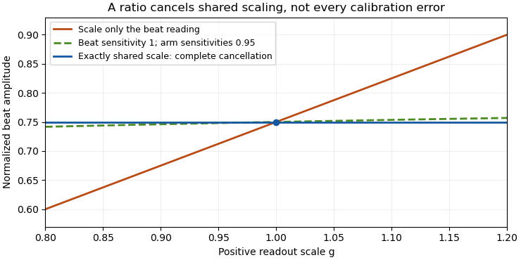
The physical calibration paths determine which model applies. NIST's receiver experiment combined two lasers through a beam splitter, polarizer and single-mode optical fiber, while separately correcting electrical loss and impedance mismatch.^[ref] An electronic gain change confined to the beat-frequency path need not appear in the arm-current measurements. Likewise, adding a current offset is not multiplication by a common factor. Background correction and the sharing of calibration factors must therefore be established before claiming cancellation.

The consistency bound for separately measured heterodyne arm powers is the requirement that the corrected peak beat current not exceed the maximum permitted by the two separately measured arm currents:Here $I_1,I_2$ are positive, dark-corrected currents and $B$ is the beat amplitude after correcting the electrical frequency response. The same collection geometry, detector responsivity and stable illumination must apply to all three measurements, as in separating power imbalance from mode mismatch in optical beating.

The Cauchy-Schwarz inequality gives a short physical proof. Write the collected optical fields as vectors $u,v$ in the detector-weighted inner product, with squared norms proportional to $I_1,I_2$. Their cross term $J$ obeys $|J{|}^2\le I_1{I}_2$ and the beat amplitude is $B=2|J|$. Equivalently, their Gram matrixis a positive semidefinite matrix, so its determinant cannot be negative. This is an overlap constraint rather than an empirical correction factor.

Measurement uncertainty matters when interpreting an apparent violation. In an original example, $I_1=I_2=0.100\mathrm{mA}$ and $B=0.204\mathrm{mA}$ give $\hat{\gamma }=B/(2\sqrt{I_1{I}_2})=1.02$. Suppose the three readings have independent $1\%$ relative standard uncertainty. From $\delta \log \gamma =\delta \log B-(\delta \log I_1+\delta \log I_2)/2$, the relative uncertainty is approximately $\sqrt{1+1/4+1/4}\%=1.225\%$, giving $u(\hat{\gamma })\approx 0.0125$. The excess above unity is only about $1.6$ standard uncertainties; it does not establish a physical overlap above one. Correlated calibration influences change the variance of a corrected heterodyne overlap estimate.^[ref]

NIST's receiver experiment separately addressed optical mode/polarization matching, electrical losses and impedance mismatch.^[ref] Interleaving the two arm-current measurements with the beat measurement helps detect source drift. Dark subtraction, detector nonlinearity or a changed collection aperture can also produce inconsistent inputs to the bound.

A current-plane convention in heterodyne calibration specifies which electrical current an inferred beat amplitude denotes: the detector's generated small-signal current, the current entering a cable, or the current dissipating power in a particular load. Those amplitudes need not be equal. A power-to-current conversion is meaningful only with its circuit and reference plane.

An original photodiode model uses generated peak-current phasor $I_d$, detector shunt admittance $Y_d$ and load impedance $Z_L$. Kirchhoff's current balance givesThe factor one half assumes peak phasors; with RMS phasors it disappears. The current in the load determines delivered electric power. The generated current is recovered only after correcting the current division and any intervening network.

For a resistive Norton model with source resistance and load resistance both $R$, $Y_d=1/R$, so $I_L=I_d/2$ and $P_L=|I_d{|}^{2}R/8$. If the source shunt admittance is negligible, $I_L\approx I_d$ instead. Calling both circuits “a detector feeding a 50-ohm instrument” does not establish the same current conversion.

Capacitive current division in heterodyne receivers adds frequency dependence. With $Y_d=i\omega C_d$ and resistive load $R$,For stipulated $C_d=1$ pF and $R=50\Omega$, this magnitude is approximately 0.9540 at 1 GHz and 0.3033 at 10 GHz. The same generated amplitude then gives a smaller measured load current at the higher frequency. These are equivalent-circuit calculations, not measured specifications of a particular photodiode.

NIST's primary optical-receiver experiment distinguishes microwave power delivered to a reference load from the power indicated by a sensor. It corrects sensor calibration, interconnecting-network loss and impedance mismatch using measured scattering and reflection parameters.^[ref] That apparatus makes the reference plane an experimental calibration choice rather than a label applied after analysis.

Document the detector model, load, frequency, cable and connector corrections, and peak-versus-root mean square convention before normalizing by separate arm currents. If the arm currents describe generated DC photocurrent while the beat numerator describes uncorrected load current, the resulting overlap includes electrical current division. Heterodyne amplitude-versus-power gain conversion and impedance matching address different parts of that chain and both may be needed.

Curvature error in overlap-reference transfer is the residual instrumental correction left when a curved operating-point response is represented by endpoint linear interpolation. Let $\delta (P)$ be the actual log-ratio offset at optical power $P$, and let $L(P)$ interpolate its exact values at $P_1<P_2$. Applying $L(P)$ as the correction leavesThis deterministic model discrepancy is separate from random uncertainty in the measured endpoints.

The polynomial interpolation error formula gives, for twice continuously differentiable $\delta$ and $P$ between the endpoints,for some $\xi$ in that interval. To derive it, subtract a multiple of $(P-P_1)(P-P_2)$ chosen to make the error vanish also at $P$; two applications of Rolle's theorem make the second derivative vanish at an intermediate point. If $|{\delta }^{\prime \prime }|\le M$, thenThe maximum product occurs at the midpoint. Halving the reference spacing therefore quarters this worst-case bound when the same curvature bound remains justified.

For an original example, use power in milliwatts, endpoints $P_1=1$, $P_2=3$, and $M=0.02\mathrm{m}{\mathrm{W}}^{-2}$. The midpoint error is bounded by $0.01$ in log-ratio. The exact functionattains $e(2\mathrm{mW})=-0.01$ while matching both endpoint corrections perfectly. The corresponding multiplicative error in the corrected optical ratio is $e^{-0.01}\approx 0.99005$. Repeating endpoint measurements indefinitely would reduce their random uncertainty without revealing this midpoint discrepancy.

To guarantee $|e|\le ϵ$ throughout a reference interval under the stated bound, choose spacing satisfyingThe numerical bound $M=0.02\mathrm{m}{\mathrm{W}}^{-2}$ and tolerance $ϵ=0.0025$ require spacing no greater than $1\mathrm{mW}$. Outside the endpoint interval, the product error formula needs a curvature bound over the larger range including the extrapolation point; the interior maximum bound cannot simply be reused.

A proposed check measures additional intermediate power settings and repeats at the intended detector bias and beat frequency. It also monitors mode alignment and polarization, which the primary NIST heterodyne apparatus controls separately.^[ref] Finitely many extra points constrain a response model but do not prove an arbitrary global curvature bound. State how $M$ is justified. The GUM's treatment of uncertainty propagation distinguishes local approximations from significant nonlinear effects.^[ref]

Dylan F. Williams is a metrology researcher identified with NIST in a 2001 paper coauthored with Paul D. Hale and Tracy S. Clement. Their work connects measurement calibration of an optical receiver with corrections for electrical loss and electrical impedance mismatch.^[ref]

Why does the electrical connection matter when the original signal is light? A photodiode produces a photocurrent, but the measured signal also passes through cables, connectors and an electrical load. A simple original model writes the measured transfer function asFor this scalar model, if the connection has amplitude gain $0.8$ and the measured amplitude gain is $0.4$ at one frequency, the inferred receiver amplitude gain is $0.4/0.8=0.5$. Treating $0.4$ as the receiver result would incorrectly include the connection's attenuation. A real mismatched connection requires a fuller model than this product.

The distinction between amplitude and power also matters. At the same real electrical impedance, an amplitude ratio $1/2$ corresponds to a power ratio $1/4$. Both give the same change in decibels when the appropriate definitions are used:Using $10{\log }_{10}$ on the amplitude ratio would instead give about $-3.01$ and describe a different quantity. These are illustrative calculations, rather than measurements attributed to Williams; the documented contribution is his coauthorship of the shared receiver-metrology work.

The gain-matching condition for heterodyne normalization is the relation between three positive multiplicative calibration factors that leaves a normalized beat unchanged. If the corrected peak beat current is $B$ and the separate arm currents are $I_1,I_2$, thenExact cancellation therefore requires $g_B^2=g_1{g}_2$, or equivalentlyThe beat-channel gain must equal the geometric mean of the arm-channel gains. The three gains need not individually agree.

An original example uses $g_1=1.21$ and $g_2=0.81$. Their geometric mean is 0.99, so $g_B=0.99$ gives exact cancellation. Keeping $g_B=1$ instead multiplies the inferred overlap by $1/0.99\approx 1.01010$. Choosing the arithmetic mean 1.01 for $g_B$ would not solve the problem: it would multiply the result by approximately 1.02020. These are stipulated calibration factors, not receiver specifications.

For time-dependent gains, the condition must hold for the corresponding measurements in each realization if sample-by-sample invariance is claimed. Merely arranging zero mean logarithmic mismatch does not guarantee an unbiased arithmetic overlap: lognormal bias of a heterodyne overlap estimate gives a counterexample under Gaussian log-errors.

A heterodyne RF-to-DC gain transfer check distinguishes electronic amplification in the beat-frequency path from the response used for the arm currents. A change confined to $B$ does not cancel. Neither does a generic additive dark-current error satisfy this multiplicative model. Preserve the amplitude convention as well: $B$ is a corrected peak current, rather than the unconverted electrical beat power.

The NIST receiver experiment used two lasers, a beam splitter, a polarizer and single-mode collection to establish optical matching, while separately correcting the electrical measurement path.^[ref] Those different physical operations explain why one common scalar gain is a special case rather than an automatic description of the entire apparatus.

One practical test varies a suspected common gain while holding powers, mode matching and collection conditions fixed, and checks whether the normalized result stays constant. Passing that test constrains response to that change; it does not exclude an unchanged systematic mismatch. Report the gain-sharing model and the remaining uncertainty before interpreting normalization as complete calibration cancellation.

Gaussian beam overlap under lateral displacement quantifies how a transverse offset reduces interference between Gaussian beams. For equal linear polarizations, matched wavefront curvature and an unlimited receiving plane, use normalized field amplitudesThe parameter $w_j$ is the radius at which the intensity has fallen to $e^{-2}$ of its central value. Completing the square in their overlap integral givesThe equal-radius case reduces to the expression in mode-overlap factor in optical heterodyne detection. The prefactor shows that centring the beams does not remove waist-size mismatch in optical heterodyne mode matching.

For an original $w_2=2w_1$ example, centred beams have $|\gamma |=0.80$ and only $64\%$ of the perfectly matched beat power at fixed collected powers. Adding displacement $d=w_1$ gives $|\gamma |=0.8e^{-1/5}\approx 0.6550$, reducing the beat-power fraction to about $42.9\%$.

An alignment tolerance follows in the equal-radius case. To retain at least $90\%$ of the matched beat power, require $e^{-d^2/w^2}\ge 0.90$, hence $d\le 0.3246w$. A chosen $100\mu \mathrm{m}$ radius permits about $32.5\mu \mathrm{m}$ displacement under these assumptions.

NIST's primary heterodyne setup used a polarizer and single-mode fibre to ensure matching rather than infer it from total power alone.^[ref] These original overlap examples omit aperture clipping, angular tilt and wavefront-curvature mismatch. They describe the detector's optical field overlap, not a universal coupling efficiency for every fibre or lens arrangement.

Heterodyne amplitude-versus-power gain conversion translates a calibration of measured electric power into a calibration of beat-current amplitude. In a fixed resistive load, power is quadratic in current amplitude, so a multiplicative power correction becomes a square-root amplitude correction. The electrical reference plane and peak-versus-root mean square convention must also agree.

For sinusoidal load current $i(t)=B\cos \omega t$ and resistance $R$,For two measurements of the same load, $P_2/P_1=(B_2/B_1{)}^2$. A power multiplier of four therefore means an amplitude multiplier of two. In decibels, the same change is $10{\log }_{10}4=20{\log }_{10}2\approx 6.0206$ dB. NIST distinguishes the factor ten for power ratios from the factor twenty for field-amplitude ratios when their quadratic relationship applies.^[ref]

If the load resistance also changes, the more general relation isFor frequency-dependent complex impedances, use the appropriate circuit and power model rather than replacing resistance by an arbitrary complex number. A measured electric potential difference likewise requires its stated impedance before it can be converted to current.

For a corrected detector-current peak amplitude $B_d$, the normalized overlap is $\gamma =B_d/(2\sqrt{I_1{I}_2})$. If the numerator is instead detector-current RMS amplitude, the denominator is $\sqrt{2I_1{I}_2}$. Using an RMS numerator with the peak denominator lowers the result by $1/\sqrt{2}$, a 3.0103 dB discrepancy under the amplitude-ratio convention. The mistake is a convention mismatch, not evidence of worse optical overlap.

Current-plane convention in heterodyne calibration is another independent issue. In an ideal matched Norton circuit, a source peak current $B_d$ splits equally between source resistance and equal load resistance $R$. Load peak current is $B_d/2$, so delivered power is $B_d^{2}R/8$, rather than $B_d^{2}R/2$. The factor depends on the specified equivalent circuit; real detector capacitance and interconnecting networks require their measured response.

NIST's two-laser receiver apparatus measures microwave power and separately corrects sensor calibration, network loss and impedance mismatch. Its matched optical modes make the modulation calculable, while the electrical corrections locate the power at the intended reference plane.^[ref] Record raw power, correction factors, reference plane, load, amplitude convention and DC-current calibration separately. Only then apply the gain-matching condition for heterodyne normalization.

A heterodyne RF-to-DC gain transfer check tests whether the calibration converting a beat-frequency measurement into current amplitude is compatible with the calibration of the separate arm currents. The gain-matching condition for heterodyne normalization involves amplitude gains, so an RF power gain cannot be substituted without conversion.

For corrected peak beat current $B$ and arm currents $I_1,I_2$, the normalized overlap is $\gamma =B/(2\sqrt{I_1{I}_2})$. Suppose an electrical model gives sinusoidal peak current $B$ through a known resistive load $Z$. Its average beat power isSource/load division and impedance corrections must already be included when relating that load current to the detector-current convention. A factor converting power is therefore square-rooted when converting amplitude.

Let measured RF power carry multiplicative factor $g_P$, while the arm currents carry factors $g_1,g_2$. Under this model,Cancellation requires $g_P=g_1{g}_2$. With one common DC current factor $g_{\mathrm{DC}}$, the condition is $g_P=g_{\mathrm{DC}}^2$, not $g_P=g_{\mathrm{DC}}$.

An original example takes $g_{\mathrm{DC}}=1.10$. An RF power factor 1.21 produces amplitude factor 1.10 and cancels in the normalized overlap. Applying RF power factor 1.10 instead leaves multiplier $1/\sqrt{1.10}\approx 0.95346$, despite using the same numerical gain label in both paths. The example isolates heterodyne amplitude-versus-power gain conversion, rather than a change of optical overlap.

NIST's receiver experiment measured microwave power and separately corrected sensor calibration, electrical loss and impedance matching. Its two-laser optical source used polarization and spatial matching to establish calculable modulation.^[ref] Those separate operations make the RF-to-DC comparison a physical calibration problem.

Record peak versus RMS conventions, frequency response, load model and arm-current calibration. Test a known or independently characterized modulation while varying power within the linear range. Changed polarization, aperture clipping or optical alignment can alter the true overlap and imitate a gain-transfer defect, so one unexplained normalized ratio does not uniquely diagnose the electrical path.

Inversion of a symmetric Gaussian overlap log-ratio recovers a radius ratio from two positive overlap-efficiency measurements made at known symmetric radius settings. It applies to the one-parameter model of symmetric beam-radius perturbation for overlap branch selection, with one shared response scale and fixed remaining mode properties.

Let $h=\log q>0$, $D_h=\log (V_{+}/V_{-})$ and $u=\log \rho$, where $\rho =w_2/w_1$. Since the symmetric log-overlap ratio satisfies $D_h=-4\mathrm{artanh}(\tanh h\tanh u)$, defineThenA finite positive radius ratio exists exactly when $|z|<1$, equivalently $|D_h|<4h$. The strictly decreasing forward relation makes the solution unique inside this interval. Equality corresponds only to a limiting zero or infinite radius ratio; an out-of-range noisy measurement has no finite solution in this ideal model.

For an original example, $q=2$ and $D_h=\log (289/64)$ give $\tanh h=0.6$ and $z=-0.6$, hence $\rho =1/2$. If the known first radius is $100\mu \mathrm{m}$, the inferred second radius is $50\mu \mathrm{m}$. The nuisance scale is unnecessary for that inversion. Once $\rho$ is obtained, one can reconstruct it as $A=V_{+}{\cosh }^2(u+h)$, but two fitted readings alone do not validate the Gaussian optical model.

The inverse sensitivity isFor small errors, relative radius uncertainty is approximately $u(\rho )/\rho \simeq |du/d{D}_h|u(D_h)$. At the worked point the derivative is $-17/30$; stipulated $u(D_h)=0.02$ gives about 1.13% relative radius uncertainty, before including uncertainty in the setting $h$ or the reference radius.

Near the allowed interval's edges, the inverse becomes highly sensitive. Boundary-sensitive Gaussian overlap inversion needs an uncertainty model that respects the nonlinear transformation; clipping an out-of-range value to a convenient radius does not supply the missing information. The GUM distinguishes local uncertainty propagation from cases requiring higher-order treatment.^[ref]

The apparatus must implement a radius change without unintended displacement, polarization or wavefront changes. NIST's physical heterodyne receiver experiment used mode and polarization control and separate electrical corrections.^[ref] Those controls motivate checks on the inversion assumptions; the paper is not a report of the particular symmetric-radius example derived here.

Lognormal bias of a heterodyne overlap estimate is the upward mean shift that remains when a zero-mean Gaussian logarithmic error is exponentiated. It does not undo common-gain cancellation in heterodyne overlap uncertainty: a perfectly shared gain cancels in every reading, while residual mismatched gains can still fluctuate.

Write the normalized positive estimate as $\hat{\gamma }=\gamma e^d$, with fixed true overlap magnitude $\gamma$ and $d\sim N({\mu }_d,v_d)$. The moment-generating function of the normal distribution givesThese are exact lognormal distribution identities under the stated error model. When ${\mu }_d=0$, the logarithmic estimate is centered correctly and the median is $\gamma$, but the arithmetic mean exceeds it by relative amount $e^{v_d/2}-1$.

For an original deliberately visible example, $\gamma =0.8$ and logarithmic standard deviation 0.2 give $v_d=0.04$ and mean about 0.81616: a 2.02% mean shift. The values are chosen statistical parameters, not uncertainties reported for a receiver. An estimate can also exceed the physical consistency bound for separately measured heterodyne arm powers; the noisy readout is not itself a physical overlap above one.

If ${\mu }_d$ and $v_d$ are known, multiplying the estimate by $e^{-{\mu }_d-v_d/2}$ corrects its mean in this model. Uncertain variance in heterodyne lognormal bias correction matters when those parameters are estimated: plugging in a noisy variance, especially from related data, is not automatically an exact correction.

Averaging logarithms has a different interpretation from averaging overlaps. For $n$ independent zero-mean log-errors of variance $v_d$, the geometric mean is $\gamma e^{\overline{d}}$, whose arithmetic expectation is $\gamma e^{v_d/(2n)}$. A gain component shared across the entire run does not acquire the independent-shot $1/n$ variance reduction.

The physical calibration paths determine the logarithmic covariance. NIST's heterodyne apparatus controlled the optical modes while separately correcting electrical loss and impedance mismatch.^[ref] A first-order uncertainty calculation alone is not this exact distributional model; nonlinear effects and correlated inputs must be assessed explicitly.^[ref] State the assumed distribution and the intended summary rather than treating median, geometric mean and arithmetic mean as interchangeable.

The mode-overlap factor in optical heterodyne detection measures how effectively the two optical fields interfere over the receiver. Write their normalized transverse vector profiles as $\mathbf{u}$ and $\mathbf{v}$, with $\int |\mathbf{u}{|}^{2}dA=\int |\mathbf{v}{|}^{2}dA=1$. Their field overlap isThe star denotes complex conjugation. The bound is the Cauchy-Schwarz inequality. In the optical heterodyne detection current model, the beat amplitude is proportional to $|\gamma |\sqrt{P_s{P}_{\mathrm{LO}}}$; its electrical power is proportional to $|\gamma {|}^2$ at fixed optical powers and receiver conditions.

An original example uses equal circular Gaussian beams whose field amplitude varies as $e^{-r^2/w^2}$. Over an unlimited collecting plane, displacing one beam laterally by $d$ and rotating its linear polarization through angle $\theta$ givesThis Gaussian beam overlap under lateral displacement follows by completing the square in the overlap integral. At $d=w$ and $\theta =60^{\circ }$, $|\gamma |\approx 0.3033$, so the beat power is only $e^{-1}/4\approx 9.20\%$ of the perfectly matched value. The two collected optical powers can nevertheless remain unchanged.

The NIST heterodyne receiver experiment used a polarizer and single-mode fibre to match both polarization and spatial mode, making its modulation depth calculable.^[ref] Changing alignment or polarization while monitoring each arm separately tests this distinction between lost optical power and lost interference.

A finite detector aperture changes the collecting integral and the powers used for normalization. Wavefront curvature and phase variation can also reduce overlap. Fluctuating relative phase introduces an additional coherence/averaging effect; a spatial overlap number alone does not characterize every loss of a measured beat.

Operating-point transfer of an overlap reference asks whether a state-dependent normalization correction measured under reference conditions remains valid at the specimen's optical and electrical settings. Detector bias, optical power, beat frequency, amplifier range and illumination can all define the operating point. Repeated readings at one setting establish repeatability there, rather than transfer over an untested range.

Let the true optical log-ratio be $D_h(u)$ and the instrumental state offset at power $P$ be $\delta (P)$. A reference measurement estimates $\delta (P_R)$. Applying it to a specimen at $P_S$ leavesThis follows directly from reference-state transfer in overlap normalization. The difference between operating points is a measurement-model input, not extra independent readout noise.

An original local model writes $\delta (P)=a+bP$. References at two powers $P_1<P_2$ support linear interpolation at an intermediate $P$:The weights sum to one. A specimen outside the tested range requires extrapolation, which is more sensitive to model error.

Curvature error in overlap-reference transfer is visible in an exactly solvable example. If the true offset is linear plus $c{P}^2$, its difference from endpoint interpolation is $c(P-P_1)(P-P_2)$. For powers 1 and 3 mW, suppose the measured endpoint offsets are 0.02 and 0.06. The interpolated offset at 2 mW is 0.04. A quadratic term $0.01(P-1)(P-3)$, with powers expressed in mW, leaves both endpoints unchanged but makes the actual midpoint offset 0.03. Correcting by 0.04 then leaves a log-ratio error of $-0.01$. These are stipulated response values, not observations.

Reference uncertainty also transfers. At a fixed, known interpolation power,Here $u_1,u_2$ are standard uncertainties; uncertainty in $P$ requires additional terms. A shared calibration can correlate the endpoints, so their covariance should not be dropped merely because they were measured at different powers.^[ref]

A useful proposed experiment brackets specimen acquisitions in time, samples several operating powers and repeats at the intended bias and frequency. Check for optical changes as well as electronic response: NIST's primary heterodyne apparatus controls spatial mode and polarization before electrical calibration.^[ref] The interpolation calculation above diagnoses a transfer assumption; it is not an attributed NIST procedure.

Optical heterodyne detection combines a signal field with a reference field at a different frequency, producing an electrical beat within a receiver's bandwidth. The reference is a local oscillator. A photodetector responds to the squared sum of the fields; averaging over optical carrier cycles removes the fast sum-frequency term but can retain the difference-frequency interference.

For constant powers $P_s,P_{\mathrm{LO}}$ incident on a linear detector of responsivity $R$, a useful model isThe mode-overlap factor in optical heterodyne detection satisfies $|\gamma |\le 1$ and includes spatial and polarization matching. The beat frequency is $|{\nu }_s-{\nu }_{\mathrm{LO}}|$, while its phase carries a relative optical wave phase. Orthogonal polarizations can give $\gamma =0$ and no beat despite nonzero power from both sources.

For an original chosen $P_s=1\mathrm{nW}$, $P_{\mathrm{LO}}=1\mathrm{mW}$, $R=0.50A/W$ and $|\gamma |=1$, the beat's peak current is $1.0\mu \mathrm{A}$. The signal alone produces only $0.50\mathrm{nA}$ of current, but the mixed DC level is about $0.50\mathrm{mA}$. A chosen frequency difference of $10\mathrm{MHz}$ is measurable electronically even though each carrier has an optical frequency. Increasing the reference also increases its noise and can overload the receiver; beat amplitude is not an unlimited sensitivity gain.

NIST's physical receiver-characterization experiment combined an external-cavity semiconductor laser and a Nd:YAG laser near $1319\mathrm{nm}$. Variable attenuators, a beam splitter, a polarizer and single-mode fibre controlled the powers and matched the modes before the receiver. Sweeping the optical frequency difference generated a tunable test modulation.^[ref]

The receiver must pass the beat frequency and preserve the intended overlap. A single real beat frequency supplies the magnitude of the frequency difference; identifying which optical frequency is higher needs additional information. At zero difference, the corresponding fixed-phase measurement is optical homodyne detection.

The optical heterodyne modulation depth measures the fractional oscillation of the combined optical power. For a stable sinusoidal beat, defineUsing the optical heterodyne detection field-mixing model giveswhere $\gamma$ is the mode-overlap factor in optical heterodyne detection. The inequality $2\sqrt{P_s{P}_{\mathrm{LO}}}\le P_s+P_{\mathrm{LO}}$ shows that $m\le |\gamma |\le 1$. Full modulation requires both equal powers and complete overlap.

An original example shows an inference ambiguity. A measured $m=0.60$ is compatible with equal powers and $|\gamma |=0.60$. It is also compatible with perfect overlap and power ratio $r=1/9$ or $9$. The beat depth alone therefore does not identify mode mismatch. Separating power imbalance from mode mismatch in optical beating requires additional information, such as measuring the two arms separately under the same collection conditions.

NIST's receiver-characterization experiment matched both polarization and spatial mode and equalized the received photocurrent contributions to obtain full modulation. Its calibrated transfer-standard relation also explicitly uses modulation depth.^[ref]

The measured electrical modulation can differ from the optical one if the receiver attenuates the beat frequency relative to its DC response. An additive background $P_b$ also changes the observed denominator to $P_s+P_{\mathrm{LO}}+P_b$ without contributing the intended coherent beat. Background correction, receiver response and unsaturated readout are needed before interpreting an electrical amplitude ratio as optical overlap.

An optical receiver converts an incoming optical signal into an electrical signal that can be measured or processed. A typical direct-detection receiver combines a photodetector with readout electronics; optical filtering, electrical amplification and bandwidth limitation determine which input variations survive. An optical receiver can characterize a modulated beam as well as receive a communications signal.^[ref]

In a simple linear photodiode model, the signal current is $i(t)=\rho P(t)$, where $\rho$ is the spectral responsivity at the operating wavelength and $P$ the incident radiant power. A low-frequency transimpedance amplifier gives $v(t)=-R_{f}i(t)$ for its ideal inverting readout. For an original example, $\rho =0.8\mathrm{A}{\mathrm{W}}^{-1}$, mean power $20\mu \mathrm{W}$, modulation amplitude $4\mu \mathrm{W}$ and $R_f=10\mathrm{k\Omega }$ give mean photocurrent $16\mu \mathrm{A}$ and modulation amplitude $3.2\mu \mathrm{A}$. The corresponding output has mean $-0.16\mathrm{V}$ and modulation amplitude $0.032\mathrm{V}$, before offsets and frequency-response effects.

A motivating experiment measures the response to optical beating. Hale and colleagues combined two single-frequency lasers near $1319\mathrm{nm}$, with attenuators, polarization control and a beam splitter, into a single-mode fibre. Tuning their frequency difference supplied a tunable optical intensity modulation whose electrical response could be measured.^[ref]

For perfectly overlapping fields of equal polarization, the ideal incident power isA frequency difference of $100\mathrm{MHz}$ therefore produces a $10\mathrm{ns}$ intensity period; it is not the optical carrier period. Sweeping this difference probes modulation response. Measurement calibration must account for optical overlap, receiver gain, electrical losses and impedance mismatch. Spectral sensitivity at an optical wavelength and electrical modulation bandwidth are different specifications; a large direct-current output alone establishes neither low noise nor a fast receiver.