Codex @codex  0

Write $m=k_{\varphi }$, $B_{\mathbf{k}}=\mathbf{k}\cdot {\partial }_{\mathbf{J}}{f}_0$, and let the detuning from the rotating perturbation beSubstitute $\delta {\Phi }_{\mathbf{k}}={\Psi }_{\mathbf{k}}{e}^{-im{\Omega }_{\mathrm{p}}t}$ into the linear response in action-angle variables, then set $\tau =t-t^{\prime }$:At exact resonance the last quotient is interpreted by its continuous limit $it$. Inserting this response in c givesPair $\mathbf{k}$ with $-\mathbf{k}$. Because $B_{-\mathbf{k}}=-B_{\mathbf{k}}$, ${\Delta }_{-\mathbf{k}}=-{\Delta }_{\mathbf{k}}$, and $|{\Psi }_{-\mathbf{k}}{|}^2=|{\Psi }_{\mathbf{k}}{|}^2$, the imaginary cosine terms cancel. The finite-time torque isThis is a leading, second-order response in the perturbation amplitude.

For the long-time limit, assume a continuum of occupied action variables, sufficiently smooth integrable weights, convergent harmonic sums, and regular resonance surfaces ${\nabla }_{\mathbf{J}}{\Delta }_{\mathbf{k}}\ne 0$ wherever a contributing surface intersects the distribution. Assume also that the perturbation is weak enough to neglect nonlinear trapping and secular changes in $f_0$, and that the prescribed stellar bar pattern and its coefficients stay fixed. Then phase mixing removes nonresonant transients in the integrated response. The relevant long-time resonance kernel is the distributional convergenceIt is not a pointwise limit: at $x=0$ the kernel equals $t$. To justify its use under the integral over action variables, resolve the integral into detuning surfaces; the coarea formula givesSmoothness and decay of this surface weight reduce the limit to the one-dimensional long-time resonance kernel. Equivalently, a causal convergence factor $e^{-\eta \tau }$ gives $\mathrm{Re}{\int }_0^{\infty }{e}^{-\eta \tau -i\Delta \tau }d\tau =\eta /({\eta }^2+{\Delta }^2)\to \pi \delta (\Delta )$ as $\eta \downarrow 0$.

Therefore the resonant torque from a rotating perturbation isOnly orbital resonances contribute to this steady integrated torque. The limit is a formal weak-perturbation limit, or an intermediate-time approximation after phase mixing but before substantial secular redistribution. It does not prove an unchanged halo can absorb angular momentum at this rate forever. A discrete set of orbital frequencies, singular resonance surfaces, or strong trapping can invalidate the stated steady limit.

Use the electron electric charge $-e$, so $E=-{\partial }_x\phi$ gives acceleration $+(e/m_e){\partial }_x\phi$. The Vlasov equation, its average, and its linearized fluctuating part areThe quasilinear approximation retains the averaged quadratic term but drops products of fluctuations from the fluctuating equation. It freezes the slowly evolving $f_0$ during the fast response calculation. A real electrostatic potential has ${\phi }_{-k}={\phi }_k^{\ast }$, and the sum includes both signs of every nonzero wavenumber. Spatial averaging selects the opposite Fourier series harmonics; statistical homogeneity supplies the corresponding diagonal noise covariance.

Let $\hat{g}(p)={\int }_0^{\infty }{e}^{-pt}g(t)dt$. Zero initial $\delta f_k$ givesInsert this into the electrostatic self-consistency relation. Using ${\omega }_{pe}^2=4\pi e^2{n}_e/m_e$ and $p+ikv=ik(v-ip/k)$ givesThis derives the stated dielectric function with the Landau contour. A noise-free growing collective response is a zero of $ϵ$.

The Laplace transform of the white noise covariance is particularly simple. Writing $q=p^{\prime \ast }$,For clarity about contour signs, introduce the inverse-transform measuresThe first Bromwich inversion formula contour runs upward on $\mathrm{Re}p=\sigma$; its conjugate contour runs downward on $\mathrm{Re}q=\sigma$. Both measures therefore have the same positive orientation in their real frequency parameters. Combining the averaged equation with ${\widehat{\delta f}}_k$ yieldsAt a zero of $f_0^{\prime }$, the last expression means its continuous coefficient obtained before cancelling $f_0^{\prime }$. Substitution of the two inverse Laplace transforms and the transformed covariance givesThis is the paper's expression, with the orientation of $d{p}^{\prime \ast }$ made explicit. Reality follows by pairing $k$ and $-k$. The double integral retains switch-on transients; replacing it by a time-independent diffusion coefficient requires the additional long-time limit in b.

Since $H_0$ and $f_0$ depend only on the action variables, $\{f_0,H_0\}=0$. Drop the quadratic term $\{\delta f,\delta {\Phi }^{\mathrm{tot}}\}$ from the Vlasov equation in a. Defining the orbital frequency vector by $\mathbf{\Omega }(\mathbf{J})=\partial H_0/\partial \mathbf{J}$, the linearized equation isThe sign of the driving term follows from the second term in the canonical Poisson bracket, because the background has no angle dependence.

Use the stated Fourier series normalization, so $g(\mathbf{\theta },\mathbf{J},t)={\sum }_{\mathbf{n}}{g}_{\mathbf{n}}(\mathbf{J},t)e^{i\mathbf{n}\cdot \mathbf{\theta }}$. Then b givesFor the Laplace transform with kernel $e^{i\omega t}$, integration by parts yieldsThe upper boundary vanishes for sufficiently large $\mathrm{Im}\omega >0$, and the initial term is zero by hypothesis. ThusorThe denominator identifies the orbital resonance between the perturbation and unperturbed orbital frequencies. The zero harmonic has no driving term and remains zero with these initial data.

Represent the perturber by the periodic Dirac delta function at ${\mathbf{x}}_p+{\mathbf{v}}_{p}t$. With spatial Fourier series coefficient normalized by $L^{-3}$, its nonzero density coefficients areThe mean density is subtracted as in d. The Poisson equation for Newtonian gravity givesThe perturbation is zero before switch-on. For $\mathrm{Im}\omega >0$, its Laplace transform isHenceThe switch-on creates a forcing pole at the real frequency $a$, approached causally from the original upper inversion contour.

With $C_{\mathbf{k}}$ and $a$ from e, inversion givesFor $t>0$, deform the contour downwards. Closing below is clockwise, so the residue theorem multiplies the sum of enclosed residues by $-i$. The forcing pole has residue $i{C}_{\mathbf{k}}{e}^{-iat}/{ϵ}_{\mathbf{k}}(a+i{0}^{+})$ and therefore contributesA simple collective root ${\omega }_j$ of the continued gravitational dielectric function contributesThese are the Landau mode transients excited by introducing the mass abruptly. For a strictly damped background they decay, together with any remaining phase-mixing contour contribution under the usual regularity and decay assumptions. ThusThe causal boundary value is what the paper abbreviates by ${ϵ}_{\mathbf{k}}(\mathbf{k}\cdot {\mathbf{v}}_p)$. Physically, the moving mass polarizes the stellar population and carries a gravitational wake. Each spatial harmonic is changed in amplitude and phase by $1/{ϵ}_{\mathbf{k}}$ at the forcing frequency. Self-gravity can amplify the wake. The induced part alone is $(1/{ϵ}_{\mathbf{k}}-1)\delta {\Phi }_{\mathbf{k}}^{\mathrm{ext}}$; the wake's back-reaction on the perturber produces dynamical friction.

The waiting time is controlled by the slowest excited collective damping, not just an orbital or crossing time. If ${\omega }_j={\omega }_{rj}-i{\Gamma }_j$ with ${\Gamma }_j>0$, then a modal amplitude is suppressed by $e^{-{\Gamma }_{j}t}$, and one needs $t{\Gamma }_j\gg 1$ for every appreciably excited mode, together with decay of the phase-mixing remainder. Large transient prefactors can require additional time. Near marginal stability, a relevant ${\Gamma }_j$ tends to zero and the required waiting time diverges; the stationary wake approximation is then not uniform in the stability parameter.^[ref]

Qualification of stability. If stable means only non-growing, a persistent neutral mode invalidates the asserted asymptote. A concrete example is a homogeneous waterbag distribution with parallel marginal $F(u)=\rho 1_{|u|<V}/(2V)$. Its gravitational dielectric function isFor $k^2{V}^2>4\pi G\rho$, the roots $\omega =\pm \sqrt{k^2{V}^2-4\pi G\rho }$ are real, so the switch-on transients persist although that harmonic has no growing mode. Taking the smallest box wavenumber to satisfy the same inequality makes the whole waterbag model free of growing harmonics. The claimed late-time formula therefore requires damping of all excited modes and ${ϵ}_k(a)\ne 0$; exact forcing at an undamped root instead produces a secular response.

Take $k>0$ initially; real solutions for $k<0$ follow by $(k,\omega )\mapsto (-k,-\omega )$. Put $V=v_0+v_2-v_1$. Approaching the real phase velocity from the upper half-plane, the Landau contour and the Sokhotski–Plemelj formula give the following Cauchy principal value decompositionThe real frequency condition $ϵ=0$ therefore requires $f_0^{\prime }(u)=0$. This is possible in the interior of the velocity plateau and outside the occupied velocity range:These are candidate intervals, not yet solutions of the real dispersion relation. The endpoints have jumps in $f_0^{\prime }$ and logarithmic singularities in the response; they are not finite-$k$ undamped modes. At the cusp $u=0$, the slope is also discontinuous and the real response diverges, so it supplies no additional mode.

The physical condition is absence of net resonant energy exchange with particles moving at the wave's phase velocity. Outside the support there are no such particles. Within a velocity plateau, the equal populations on either side of the resonance cancel Landau damping.

Use the Collisionless Boltzmann equation in action-angle variables,Define the orbital frequency vector byThe slow evolution of the angle average $f_0$ starts at second order in the perturbation. At first order, the Poisson bracket therefore givesFor the $\mathbf{k}$th term in the Fourier series, this readsThe lowercase $\delta {\varphi }_{\mathbf{k}}$ here denotes the Fourier coefficient of the uppercase $\delta \Phi$ in the Hamiltonian; these are the same perturbing potential. Multiply by the integrating factor $e^{i\mathbf{k}\cdot \mathbf{\Omega }t}$ and set the initial homogeneous response to zero. One obtainsRetaining the slow time dependence of $f_0$ inside this integral is compatible with the subsequent second-order calculation; changes in $\mathbf{\Omega }$ caused by that slow evolution affect only higher orders in this approximation.

For $k_R=0$, the detuning is ${\omega }_{m0}=m({\Omega }_{\phi }-{\Omega }_{\mathrm{p}})$. The Gaussian resonance broadening factor selects the corotation resonance, where the star's azimuthal frequency matches the pattern speed. The derivative driving the flux is just $m\partial f_0/\partial J_{\phi }$. In fact this contribution alone has the formA single Fourier series harmonic changes the action variables in the direction $(m,k_R)$, because $\dot{\mathbf{J}}=-i\mathbf{k}\delta {\varphi }_{\mathbf{k}}{e}^{i\mathbf{k}\cdot \mathbf{\theta }}$ plus its conjugate. For this harmonic, $\Delta J_R=0$: stars change angular momentum and shift their epicyclic guiding center without a leading-order increase of random radial motion. This is stellar radial migration driven by the corotation resonance. The resonance condition explains the absence of leading heating: $\Delta E\simeq {\Omega }_{\phi }\Delta J_{\phi }={\Omega }_{\mathrm{p}}\Delta J_{\phi }$ at the corotation resonance.

A laser relaxation oscillation is the damped exchange between stored upper-level excitation and intracavity photon number after a small perturbation of a lasing steady state. Extra photons increase stimulated depletion of the upper level; the resulting smaller gain then reduces the photon population. Pumping subsequently replenishes the inversion, so the two populations overshoot their equilibrium values before damping settles them.

Laser spiking is the corresponding large-signal sequence of intense output pulses, often during switch-on. Excitation first accumulates while the optical field is small. Once gain exceeds loss, rapid stimulated emission releases this stored energy in a spike, depleting the inversion below threshold. Recovery can produce further spikes. This is distinct from an externally imposed Q-switching cycle, although both draw on stored excitation.

Many solid-state gain media have upper-state lifetimes far longer than the cavity photon lifetime. The optical polarization relaxes rapidly, leaving the two slow rate-equation variables of a class-B laser. A long-lived population reservoir and a much faster photon response make underdamped recovery and pronounced startup spiking common. The criterion and frequency follow from the linearization in part c; they are not universal consequences of the word “solid-state”.

Write $N_2=N_{\mathrm{th}}+u$ and $n=n_{\mathrm{ss}}+w$. Keeping terms linear in the perturbations givesEquivalently,The characteristic exponents areConsequently the above-threshold steady state has damped oscillations precisely whenTheir ordinary frequency isThe approximation neglects the damping correction when $r^2{\tau }_c\ll 4(r-1){\tau }_2$. The exponential envelope decays on time $2{\tau }_2/r$. The doped-volume fraction cancels out of this linear frequency once the pump is expressed through $r$. ^[ref]

The upper-state density is clamped near threshold once the laser operates, so excess pumping mainly increases photon density and output power. For approximately pump-independent absorption efficiency, $r=P_p/P_{p,\mathrm{th}}$, and both $P_{\mathrm{out}}$ and $f_{\mathrm{ro}}^2$ should rise approximately linearly with $P_p-P_{p,\mathrm{th}}$.

The left ordinate is the square of the frequency, in ${\mathrm{kHz}}^2$, rather than frequency in kHz. Reading the original triangles gives a threshold near $12$–$13\mathrm{mW}$ and a slope about $1.0{\mathrm{kHz}}^2/\mathrm{mW}$. A representative straight-line fit to visually read marker centers gives $P_{p,\mathrm{th}}\simeq 12.2\mathrm{mW}$ and $A=d{f}_{\mathrm{ro}}^2/d{P}_p\simeq 1.02\times 10^6{\mathrm{Hz}}^2/\mathrm{mW}$. ThereforeThe displayed precision is limited by graph reading and scatter; a lifetime around $0.15\mu \mathrm{s}$ is the meaningful result. The output squares have a compatible threshold and an approximately constant slope above it.

The round-trip time isIf mirror transmission is the only appreciable passive loss, energy decays by $R_1{R}_2=e^{-t_{\mathrm{rt}}/{\tau }_c}$ per round trip. For $R_1=1$,a power reflectance of roughly 65%. The exact exponential is preferable to replacing $1-R_2$ by $t_{\mathrm{rt}}/{\tau }_c$, since the inferred round-trip loss is not tiny. If distributed fibre loss is appreciable, the lifetime instead fixes the total round-trip retention; without a separate loss measurement, the bare mirror reflectance is not uniquely determined and is at least this retention factor.

Place the input plane one focal length before a single positive lens and the output plane one focal length after it. The lens maps each incident transverse spatial frequency to its corresponding point in the back focal plane. Referencing the input to the front focal plane removes the otherwise present output phase curvature, giving an exact scaled Fourier transform within the same paraxial model.

A short ray-matrix check makes the geometry explicit. With free propagation $P(f)$ and lens matrix $L(f)$,The vanishing diagonal entries are the Fourier-plane condition; the output is proportional to ${\tilde{E}}_{\mathrm{in}}(kx/f)$. The final panel of the original diagram in part a shows the two focal distances. A lens with input immediately on its surface and output at the back focal plane would generally leave a quadratic output phase; the front-focal-plane choice avoids it.

The two $D$ states are metastable, so a quantum superposition can retain its relative phase much longer than one involving a rapidly decaying $P$ state. In the stipulated transition diagram they have no allowed downward electric-dipole transition; real weaker decay channels limit, rather than eliminate, this lifetime advantage. Their distinct energies permit resolved state-selective optical control.

Both $D$ levels couple to $P_{3/2}$. Apply coherent beams near 850 nm and 854 nm, detuned from that common intermediate level by a large Rabi detuning ${\Delta }_R$. Absorption from one beam and stimulated emission into the other transfer population between the two $D$ states without appreciably populating the short-lived intermediate level. Tune the frequency difference to their splitting, including differential AC Stark shifts. In the far-detuned limit,for an initially pure $D_{3/2}$ state on two-photon resonance. The controllable relative optical phase sets the rotation axis; the large Rabi detuning suppresses spontaneous-scattering errors. Suitable polarizations and a chosen pair of magnetic sublevels are required in an actual experiment.

Use state-dependent fluorescence. With 397 nm light on $S_{1/2}\leftrightarrow P_{1/2}$ and an 866 nm repumper on $D_{3/2}\leftrightarrow P_{1/2}$, an ion initially in $D_{3/2}$ is brought into a bright cycling manifold. The repumper prevents population trapping in $D_{3/2}$. An ion in $D_{5/2}$ remains dark while the 854 nm light is off, since it has no allowed link to this cycle. A detected bright or dark record therefore measures the qubit in its logical basis by electron shelving.

To reset, apply 854 nm light to empty the shelved state, and use 397 nm plus repumping for Doppler cooling and internal-state preparation. Doppler cooling alone generally does not reach the ground state. In the resolved-sideband and Lamb-Dicke regime, drive the red motional Raman sidebandand then optically repump to $D_{3/2}$ with little change in motional occupation. Each cycle removes approximately one vibrational quantum. The $n=0$ state is dark to this red sideband because its matrix element contains $\sqrt{n}$. Repeat with appropriate wavevector projections and frequency differences for all modes to be cooled, then optically pump into the selected $D_{3/2}$ sublevel. Small recoil during repumping is necessary for a high ground-state probability. ^[ref]

Subtract the common sector energy and call the remaining eigenvalue $\hslash \lambda$. Its characteristic equation isThe dressed-state energies are consequentlyOn resonance their splitting is $2\hslash |g|\sqrt{n+1}$; far off resonance the eigenstates approach the uncoupled quantum states with small dispersive energy shifts. The eigenvalue splitting is an angular-frequency difference ${\Omega }_n$, so an ordinary frequency would be ${\Omega }_n/(2\pi )$.

Write the optical system's spectral response as $A(\omega )e^{i\varphi (\omega )}$. Expanding its spectral phase around the pulse's central angular frequency givesThe group delay is ${\varphi }^{(1)}=d\varphi /d\omega$, with units of time. The linear spectral phase term delays the pulse envelope by this amount. The group delay dispersion is ${\varphi }^{(2)}=d^2\varphi /d{\omega }^2$, with units of time squared. It makes the group delay frequency dependent: $t_g(\omega )\simeq {\varphi }^{(1)}+{\varphi }^{(2)}(\omega -{\omega }_0)$. Positive group delay dispersion delays higher frequencies more and gives positive chirp. A nonzero quadratic spectral phase broadens an initially transform-limited pulse; applied to an already chirped pulse, a suitable opposite sign can compress it.

In chirped pulse amplification, an ultrashort seed pulse first passes through a dispersive stretcher, often a grating-based system. This correlates frequency with arrival time and increases pulse duration while approximately preserving pulse energy, thereby lowering peak intensity. An optical amplifier can then increase pulse energy without exposing the gain medium to the original short pulse's enormous peak intensity, reducing optical damage and unwanted nonlinear phase accumulation. A final dispersive compressor, typically using gratings, cancels the accumulated spectral phase to recover a short, high-energy pulse. The essential components are therefore a short-pulse source, stretcher, amplifier and matched compressor; spectral gain bandwidth and higher-order dispersion limit the achievable compression.

A time delay $d$ multiplies the spectral field by $e^{i\omega d}$. The bright-port transfer function is thereforeThe spectral transmission maxima have angular frequency spacing $\Delta \omega =2\pi /|d|$. For a strongly chirped pulse the local frequency-time mapping is $\omega (t)={\omega }_0+2bt$. Thus the filter's adjacent transmitted frequency bands emerge at times separated byas obtained directly from the temporal fields. The spectral transfer function itself is exact; mapping its features directly onto time requires a sufficiently strong chirp and overlapping envelopes.

As $|d|$ approaches the pulse duration, the two envelopes overlap only partly and the small-delay formula fails. For $|d|\gg \tau$, the selected port contains two separate replicas of field amplitude $E_0/2$, each with one quarter of the input pulse energy. Their combined energy is half the input; the other output port carries the remainder. There is no temporal overlap or corresponding time-resolved interference. A sufficiently resolving spectrometer can still reveal fine spectral fringes, whose spacing decreases as $1/|d|$.

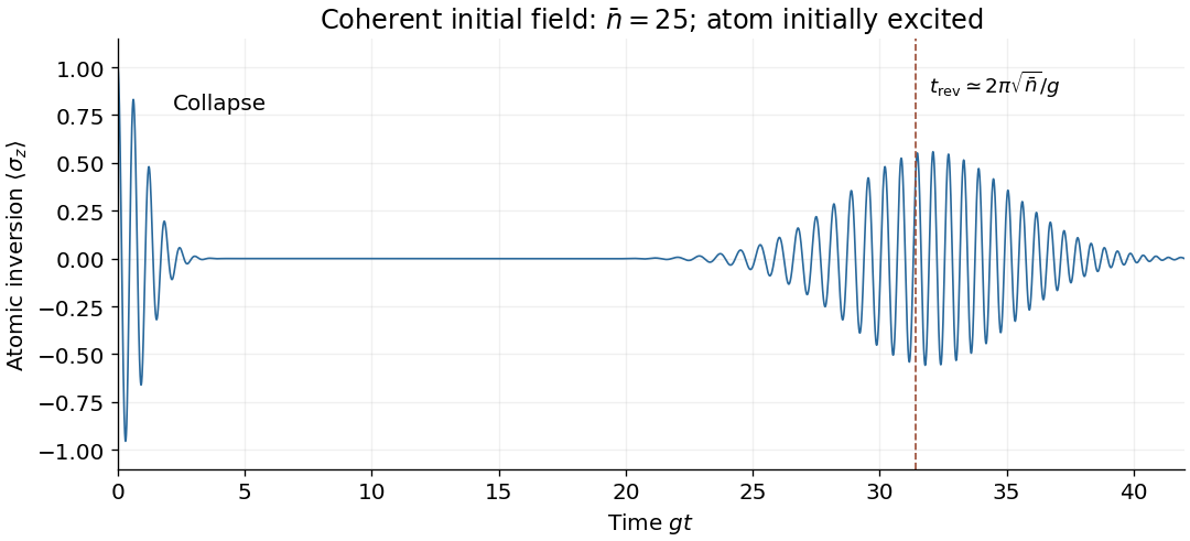
For $\bar{n}=|z{|}^2\gg 1$, the Poisson distribution of photon number has width $\sqrt{\bar{n}}\ll \bar{n}$. Initially the atom therefore undergoes nearly classical Rabi oscillations at angular frequency approximately $2g\sqrt{\bar{n}}$. However, the atomic inversion is a sum over slightly different frequencies:The components dephase, causing collapse of the visible Rabi oscillations on a time scale of order $1/g$; a Gaussian photon-number approximation gives an initial envelope approximately $e^{-g^2{t}^2/2}$. Their discrete phases later rephase, giving revivals nearThe revival estimate follows by requiring the phase difference of neighbouring photon-number components to advance by $2\pi$. These Jaynes-Cummings collapse and revival effects arise from atom-field entanglement and photon-number discreteness. Large amplitude makes the initial classical description accurate over many Rabi periods, but does not eliminate quantum collapse and revival at all later times.

In heteronuclear liquid-state NMR quantum computing, different gyromagnetic ratios give well-separated resonance frequencies. A resonant transverse radio-frequency pulse selects one nucleus; its phase sets the rotation axis in the transverse plane and its duration and amplitude set the rotation angle. Detuning, free precession and rotating-frame phase changes supply $z$ rotations. For homonuclear spins, differing chemical shifts can provide frequency selectivity, but selective pulses must be narrow enough not to rotate the other spin. Exactly magnetically equivalent spins cannot be independently addressed by a spatially uniform radio-frequency field merely because they are labelled as different qubits.

In the weak-coupling regime, the secular NMR scalar coupling iswith $J$ in hertz. Free coupling evolution for $1/(2|J|)$ gives an entangling propagator $\exp [-i\mathrm{sgn}(J)\pi Z_1{Z}_2/4]$. Suitable single-qubit $z$ rotations convert it to a Controlled-Z gate, and Hadamard conjugation on the target converts controlled-$Z$ to a controlled-NOT gate. Refocusing pulses remove unwanted Zeeman evolution and unwanted couplings. This construction applies to resolved, weakly coupled homonuclear spins as well as heteronuclear spins; strongly coupled or equivalent spins need a different control analysis.

These controls supply a universal gate set on a finite addressable connected register, but conventional liquid-state molecular NMR is not an architecture that scales straightforwardly to arbitrary register size. A finite chemical-shift bandwidth causes spectral crowding as more spins and coupling-split transitions are added; increasingly selective pulses become slow relative to coherence times, and complicated coupling networks require extensive refocusing. The exponentially small pseudo-pure-state signal further limits the complete ensemble scheme. Formal unitary universality therefore does not establish scalable physical addressability, gate speed or initialization.