Nuclear magnetic resonance detects the response of atomic nuclei with a magnetic moment to a radio frequency magnetic field in a steady magnetic field. Its striking possibility is to measure a nuclear property through an ordinary electrical signal from a bulk sample: an enormous number of tiny magnetic moments can produce a measurable change in a receiving circuit.
For a nucleus with spin angular momentum , define its gyromagnetic ratio by . Throughout this article is angular, measured in radians per second per tesla; is the corresponding value in cycles per second per tesla. With , the Hamiltonian is . Adjacent energy levels differ byThus a measured resonance frequency and a calibrated magnetic field determine . Converting that into a nuclear magnetic moment also requires the spin quantum number: the maximum projection has magnitude . This simple experiment does not by itself determine the sign of .
The Rabi molecular beam magnetic resonance experiment detects transitions through changes in a selected molecular beam. The bulk experiments below instead detect electrical consequences of nuclear magnetization in matter at ordinary density. A small Boltzmann distribution population imbalance is multiplied by a very large number of nuclei. For noninteracting spin one-half nuclei of number density and positive , their equilibrium magnetization isThis follows by weighting the two projections with their Boltzmann distribution probabilities. It explains both the smallness of the bulk polarization at ordinary temperature and the value of many nuclei contributing to one receiving circuit.
NMR spectroscopy measures resonant responses of atomic nuclei to applied electromagnetic radiation in a magnetic field. In residual-group monitoring of polyurethane formation, distinguishable signal integrals supply a relative residual-group readout; overlap or very weak signals can limit that inference.
Spectroscopic measurement of tissue chemical signals, complementary to anatomical magnetic resonance imaging.
The number and relative intensities of lines into which an NMR signal is split by scalar spin coupling.
nuclear magnetic resonance of the spin-one-half isotope . Equivalent silicon sites give the same isotropic chemical shift, while condensation and silanol substitution can distinguish environments. Line heights alone are not quantitative populations.
A spin system with two distinguishable, mutually coupled spins A and B, each coupled to three equivalent X spins. An ethoxy methylene with nonequivalent hydrogens can display this pattern; small A/B chemical-shift separation relative to their coupling produces second-order distortion.
For the two-spin Hamiltonian operator , juxtaposition of two Pauli matrices denotes their tensor product. Put . The exchange matrix element between and is , whereas their diagonal separation is . Nondegenerate perturbation theory therefore gives admixtures and second-order frequency shifts . Neglecting the exchange terms is justified to leading order when . A large common Zeeman energy is insufficient. To approximate accumulated phases by this leading-order Hamiltonian operator, one also needs over the observation time, or must include the second-order shifts.
For fixed nonidentical chemical shifts, increasing the static magnetic field increases in angular-frequency units while the NMR scalar coupling changes little. If remains exact, the approximation fails at every nonzero .
The leading-order averaging of rapidly oscillating exchange terms in the interaction picture of two nuclear Zeeman energy terms. For ,Their first-order time integrals are bounded by , so they contribute little when , while the stationary Ising coupling survives. Higher orders give frequency shifts of order . This approximation is controlled by the difference of resonance frequencies, not their common magnitude.
Coupled relaxation of nuclear-spin populations through their mutual interactions.
reduction of a resonance linewidth when motion averages otherwise distinct local magnetic environments. The onset probes a motional timescale but does not by itself establish long-range transport.
The decay timescale of the local magnetic-field fluctuations that relax a nuclear spin. Its relation to a tracer jump waiting time depends on geometry and the microscopic stochastic model.
A polarization-transfer carbon NMR experiment giving opposite phases to CH-two versus CH/CH-three signals in its usual convention; nonprotonated carbons are absent. Combined with other spectra it distinguishes methylene, methyl/methine and quaternary sites.
Heteronuclear multiple-bond correlation: an experiment commonly detecting proton-carbon scalar coupling across two or three bonds. Occasional longer-range peaks, missing peaks and intensity variations require cautious interpretation.
Heteronuclear single-quantum coherence: a two-dimensional experiment commonly correlating a proton with its directly bonded carbon through one-bond scalar coupling.
Correlation spectroscopy: a two-dimensional proton NMR experiment whose cross peaks identify scalar-coupled proton pairs. Overlap can prevent a unique letter-by-letter assignment.
Nuclear magnetic resonance using lithium isotopes. Lithium-6 has spin 1 and a small quadrupole moment, often giving narrower aggregate resonances than lithium-7.
The timescale relevant to resolving exchange between resonance frequencies. Fast and slow are relative to the frequency separation and measurement, not absolute labels for molecular motion.
Imaging based on spatial encoding of nuclear magnetic resonance signals. Acquisition and reconstruction choices determine which physical contrasts can be measured.
An imaging approach describing direction-dependent water diffusion using a tensor model. In white matter it provides indirect information about tissue organisation; crossing fibres, motion and model limitations affect interpretation.
A dimensionless measure of dispersion among the diffusion tensor eigenvalues. With eigenvalues and mean , when the denominator is nonzero. It is not a direct measure of axon number or functional necessity.
Magnetic-resonance measurements sensitive to water diffusion. Models of directional diffusion can support tractography, subject to limitations such as crossing fibers, partial volume and modeling assumptions.
Estimation of plausible pathways from diffusion measurements and modeling choices. Reconstructed streamlines are not a direct count of axons and do not by themselves determine synaptic direction, signal flow or functional necessity.
Imaging task-related or spontaneous changes in magnetic-resonance signals associated with physiology, commonly the BOLD signal. Hemodynamic timing and spatial averaging constrain inferences about neural firing and cell-level computations.
A magnetic-resonance signal sensitive to blood oxygenation and related vascular changes. It is an indirect correlate of local neural processing, with slower dynamics than individual spikes.
An ideal resonant inversion pulse reverses the longitudinal magnetization. Subsequent spin-lattice relaxation gives the displayed recovery law. Observation at a chosen inversion time provides contrast or nulling for a specified relaxation time; an RF inversion alone does not amplify the initial polarization magnitude.
Magnetic resonance imaging with a prepared nuclear population imbalance exceeding ordinary thermal polarization under the imaging conditions. Dynamic nuclear polarization, optical spin transfer and spin-order transfer offer different preparation routes. Preparation and acquisition must account for spin-lattice relaxation, which erases the excess polarization.
The spatial Fourier-frequency coordinates sampled by a magnetic-resonance acquisition. With gyromagnetic ratio in radians per time per field, the displayed expression is in cycles per length. Signal phase, gradient history and sequence refocusing determine the trajectory; the samples require reconstruction to form a spatial image.
A detection probe with cooled electronic components to reduce noise and improve sensitivity. The sample need not itself be cooled to the electronics temperature.
Transfer of polarization from electron spins to nuclei to enhance NMR sensitivity. Added radicals and low-temperature conditions can alter spectral resolution and the states sampled.
NMR measurements on immobilized or slowly moving samples, using approaches such as decoupling, sample alignment or magic angle spinning to manage anisotropic interactions.
Sample rotation about an axis at approximately to the field, averaging appropriate second-rank anisotropic interactions when spinning and pulse conditions are suitable.
Additional nuclear relaxation associated with a paramagnetic centre. With appropriate controls, its distance dependence constrains molecular arrangement and transient contacts.
A coupling remaining when orientational averaging of a dipolar interaction is incomplete. It can constrain bond-vector orientation in a suitable alignment frame.
A change in one nuclear signal caused by perturbing another through cross-relaxation. Appropriate measurements constrain distances or molecular motions, with interpretation dependent on dynamics.
Transfer of magnetization through a network of coupled spins, which can create indirect NOE correlations.
Rotating-frame Overhauser effect spectroscopy, using NMR cross-relaxation during a spin-lock period.
Two-dimensional nuclear Overhauser effect spectroscopy, detecting NMR cross-relaxation between nuclear spins.
Evolution of nuclear-spin populations and coherences toward equilibrium. Different relaxation measurements report different aspects of molecular motion.
NMR methods selecting slowly relaxing coherence components through interference between relaxation mechanisms. Appropriate labelling and field conditions extend measurements to larger assemblies.
Methyl-based NMR strategies exploiting favourable relaxation properties of selected methyl coherences, often with selective isotopic labelling in a largely deuterated protein.
Chemical exchange in NMR interconverts environments during the observation. Fast exchange relative to their frequency difference produces averaged shifts; slow exchange resolves separate sites. A single peak alone does not prove a single static geometry.
Exchange much faster than the resonance frequency difference gives one population-weighted resonance. The averaging does not prove a single static geometry.
Boron-11 nuclear magnetic resonance probes boron environments. Rapid exchange can average inequivalent sites into one resonance; slow exchange reveals distinct sites. Quadrupolar relaxation and line broadening can complicate integration.
Phosphorus-31 nuclear magnetic resonance observes spin-one-half phosphorus-31. An system can show a two-phosphorus doublet and a one-phosphorus triplet; three inequivalent mutually coupled phosphorus sites can each give a doublet of doublets in the first-order limit.
Proton nuclear magnetic resonance measures resonances of hydrogen-1 nuclei. Structural signal counts require an explicit symmetry and exchange-timescale model; exchangeable N–H or O–H signals can be broadened or lost.
NMR observation of spin- fluorine-19 nuclei. Coupling to nearby protons can split a resonance unless proton decoupling is applied.
NMR observation of spin- carbon-13 nuclei. Routine spectra often use proton decoupling, but this does not automatically decouple other spin-active nuclei.
An NMR multiplicity-editing experiment in which carbon signals are separated by the parity of their attached proton count: CH and CH3 have one relative phase, while CH2 and nonprotonated carbons have the other. The absolute up/down convention depends on processing and is not a universal assignment.
Irradiation that removes resolved scalar spin-spin coupling to protons from another nucleus’s spectrum. Other couplings, such as carbon–fluorine coupling in a proton-decoupled carbon-13 NMR spectrum, can remain.
The area of a resonance or multiplet, proportional to the contributing nuclear population under suitable excitation, relaxation and acquisition conditions. Relative proton integrals can count chemically distinct protons.
Through-bond interaction between nuclear spins that splits NMR resonances. In the weak-coupling limit, equivalent spin- neighbours produce lines with binomial coefficient intensities. Equivalent nuclei do not split each other.
Proton coupling across H-C-C≡C-H can resolve a small four-bond splitting. In a propargyl acetal this connects the acetal methine and terminal alkyne proton.
Through-bond spin coupling involving vinylic nuclei. The geometry of a vicinal pathway across an alkene distinguishes cis and trans coupling.
vicinal coupling between protons on the same side of an alkene. A measured first-order splitting is an approximation if the spin system is appreciably strongly coupled.
vicinal coupling between protons on opposite sides of an alkene. In many ordinary terminal alkenes its magnitude exceeds the corresponding cis coupling.
A set of resonance lines arising from resolved spin coupling. Weak-coupling patterns can be assigned through coupling paths and line intensities; line count alone can be ambiguous.
An approximately six-line scalar-coupling pattern. Similar coupling to five spin-one-half partners can mimic a sextet even when those partners are not all chemically equivalent.
A first-order NMR multiplet produced by coupling to two distinct sets of three equivalent spin-one-half nuclei. Sixteen lines are possible; equal couplings can collapse the pattern to a septet.
A first-order NMR multiplet split into a doublet by one spin-one-half nucleus and into quartets by three equivalent spin-one-half nuclei. Ideally it has eight lines; overlap and second-order behavior can change its appearance.
A first-order NMR multiplet split successively by two distinct spin-one-half couplings and by two equivalent spin-one-half nuclei. Ideally it has twelve resolved lines before coincidences or further unresolved couplings.
A seven-line First-order NMR multiplet. Coupling to six equivalent spin-one-half neighbours gives the intensity ratio .
A four-line first-order pattern, often from three equivalent spin-one-half neighbours, with intensities 1:3:3:1. Equal couplings to different groups can mimic it.
A three-line first-order pattern, often from two equivalent spin-one-half neighbours, with intensities 1:2:1.
A pair of lines with the first-order splitting expected for one spin-one-half neighbour. Additional unresolved or coincident interactions can complicate the pattern.
A resonance with no resolved scalar splitting under the acquisition conditions. This does not prove that every coupling is exactly zero.
Through-bond coupling over a longer path, often four or more bonds. Small resolved allylic couplings can split alkene and oxygen-bound methylene signals and should not be discarded merely because vicinal couplings are larger.
Coupling across an allylic four-bond path, such as between an oxygen-bound CH2 group and terminal vinyl hydrogens in an allyl ester.
The line pattern obtained when chemically distinguishable spin groups can be treated in the weak-coupling approximation. For an observed spin, each coupled neighbour contributes a frequency displacement of plus or minus half the relevant coupling; coincident lines add intensities.
A first-order pattern combining a doublet splitting with a triplet splitting, commonly from one neighbour and a pair of equivalent neighbours.
Splitting by two distinguishable spin-one-half neighbours with different resolved coupling magnitudes. The four line positions are displaced from the centre by every choice of plus or minus half of each coupling.
Four equally spaced lines can arise from three equivalent neighbours or from coincident couplings to different groups. Combining a doublet with a triplet of the same spacing gives intensities 1:3:3:1; line count alone does not identify a unique topology.
The frequency spacing of a first-order multiplet, expressed in hertz. For a spectrum at MHz, . A bond-count superscript, such as , specifies the coupling path.
A Karplus equation relates a vicinal scalar coupling to molecular torsion, often represented as . Parameters depend on the chemical environment. A mobile molecule gives a population average of couplings, which is generally not the coupling evaluated at its mean angle.
NMR relaxation dispersion measures how an observed nuclear-spin relaxation rate changes with pulse timing or effective field conditions. Models can constrain exchange between molecular environments, including weakly populated conformations; rate and population estimates depend on the exchange model and information content.
A chemical shift measures an NMR resonance position relative to a reference. Electronic environments alter local magnetic shielding, so shifts can report a changed molecular environment without uniquely specifying a structure.
Nuclei with the same resonance frequency in the specified environment. Equivalent chemical shifts do not automatically imply magnetic equivalence when couplings to other nuclei differ.
The chemical-shift position around which a first-order multiplet is split. A labelled outer line is not generally the resonance centre.
Dependence of nuclear shielding and resonance frequency on molecular orientation relative to the magnetic field. Its modulation contributes to nuclear-spin relaxation.
In their 1946 letter, Felix Bloch, William Webster Hansen, and Martin Packard reported water at room temperature. A steady magnetic field along and an oscillating field along produced a signal in a pickup coil along , displayed on an oscilloscope. Some samples included paramagnetic additives to accelerate thermal equilibrium. Resonance fields at two frequencies gave the same field-to-frequency ratio, consistent with the proton value.[ref]
Nuclear Induction by Felix Bloch and others. p. 127, Nuclear Induction, entire letter; geometry, water, additives, readout and two-frequency check
The detailed paper describes glass water bulbs inside tuned receiving coils. Transmitter coils, shields and a conducting paddle controlled leakage. Field modulation at 60 Hz drove the horizontal oscilloscope sweep. A diode and audio amplification supplied the vertical trace. Vibration changed coupling: their largest difficulty. Coil tuning capacitors formed tank circuits. The actual receiver omitted the conceptual diagram's radiofrequency amplifier.[ref]
The Nuclear Induction Experiment by Felix Bloch and others. pp. 475–480, Figs. 1–4, APPARATUS and opening RESULTS; actual diode receiver versus conceptual amplifier
The orthogonal coil axes suppress direct transmitter pickup, but do not eliminate it. A field-dependent signal at the nuclear resonance must be distinguished from leakage and noise; merely detecting a radiofrequency voltage is insufficient. This is why the field sweep and the independently checked field-to-frequency ratio matter.
Edward Mills Purcell, Henry Cutler Torrey, and Robert Vivian Pound placed paraffin wax in a capacitively loaded coaxial cavity near 30 MHz between magnet poles. Coupling loops supplied and extracted power; oscillating and steady fields were perpendicular. Output balanced against a generator reference fed amplification, detection and a microammeter. A slow field sweep revealed absorption above fluctuations at room temperature. Weak drive avoided population equalization. Calibration was rough; field inhomogeneity could contribute to linewidth.[ref]
Resonance Absorption by Nuclear Magnetic Moments in a Solid by Edward Mills Purcell and others. pp. 37–38, apparatus and results; weak drive, balanced cavity output, microammeter, field sweep, calibration and linewidth limitations
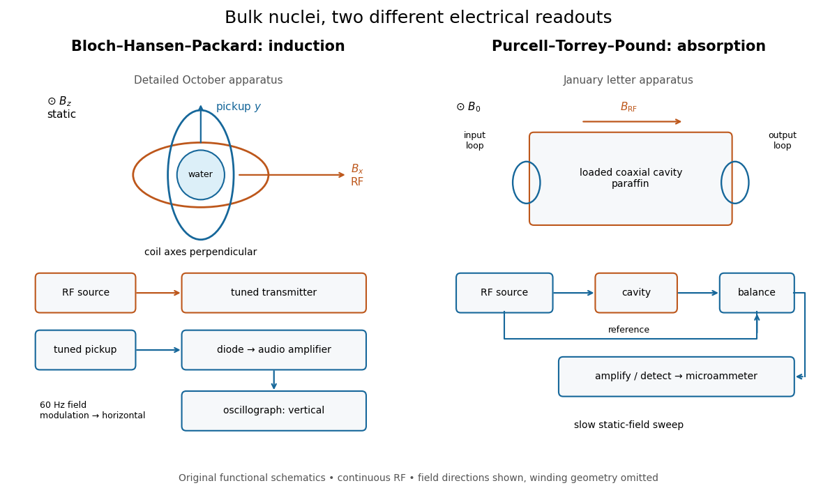
Two electrical routes to bulk nuclear magnetic resonance
. Original functional diagrams of the distinct instruments described above. Arrows show connections and field directions, not scale or winding geometry. Details.These are driven experiments with continuous radiofrequency excitation and changing static field, not demonstrations of modern pulsed Fourier transform nuclear magnetic resonance. Bloch's theoretical paper explicitly distinguishes proposed free precession after a pulse from the forced precession actually studied.[ref]
Nuclear Induction by Felix Bloch. pp. 460–461, introduction: proposed pulse/free-precession experiment versus performed forced-precession experiment
An experimental failure need not mean absent nuclear magnetic moments. In the model below, excessive drive reduces the population imbalance through nuclear magnetic resonance saturation; waiting too briefly can leave insufficient polarization. Separately, ordinary electrical losses can cause heating without identifying a nuclear resonance. The absorption experiment measured a balanced electrical signal, rather than using heating as its readout. Useful diagnostic checks include moving off resonance, changing the frequency, checking field uniformity and reducing drive. These are general checks; the historical operations actually documented are specified above.
The Bloch equations describe an ensemble magnetization with Larmor precession plus phenomenological recovery and decay:Here are model parameters, not a microscopic explanation of relaxation. The precession term follows from the torque on a magnetic moment; the two dissipative terms prescribe exponential decay. Bloch explicitly introduced this macroscopic relaxation description as a simplifying approximation.[ref]
Nuclear Induction by Felix Bloch. §4, pp. 467–468, equations (32), (37) and (38): longitudinal recovery and assumed exponential transverse decay
For positive and no transverse drive, rotates as : its signed rotation is negative about , although the resonance angular frequency is positive. This distinction prevents a hidden sign change when choosing a rotating frame.
With no transverse drive, the Bloch equations giveLongitudinal nuclear spin relaxation restores the population imbalance and thus the magnetization parallel to the static magnetic field. It corresponds to population relaxation for the two-level model. Starting from , waiting recovers of , whereas waiting recovers about . This is why repeated measurements require a recovery-time decision.
Transverse relaxation describes loss of ensemble transverse magnetization. It must not automatically be identified with pure dephasing. In a simple completely positive two-level relaxation model,where describes additional pure dephasing. Thus population recovery itself contributes to transverse decay. A spread of static magnetic fields can further cancel ensemble phases without the same microscopic relaxation; an observed free signal may have an effective rather than homogeneous . The simple exponential examples below assume a uniform field and a single homogeneous .
Free induction decay is a receiving signal from freely precessing transverse magnetization after excitation ends. Faraday's law of induction gives coil voltage proportional to the time derivative of linked magnetic flux, with sign set by the winding. At its envelope follows the transverse magnetization; a fixed receiver phase can absorb the derivative's near-quadrature shift. We define the calibrated complex signal below to represent magnetization, not raw coil voltage.
For an original teaching model, take positive , a circular drive , and axes rotating at about . Define , , and . The Bloch equations becomeA linearly oscillating field of peak amplitude has a co-rotating component of amplitude ; neglecting its counter-rotating component requires near resonance.
At resonance, a short pulse starting from gives with , neglecting relaxation during duration . A receiver phase rotation can make a pulse's initial transverse signal real. After the pulse, direct integration givesThese are the two components extracted by quadrature demodulation. Differentiating verifies ; taking its magnitude separates decay from detuning.
Choose rounded illustrative , , , and . Then and the duration is , short relative to both relaxation times. For receiver detuning and , and . These are calculated examples, not 1946 measurements.
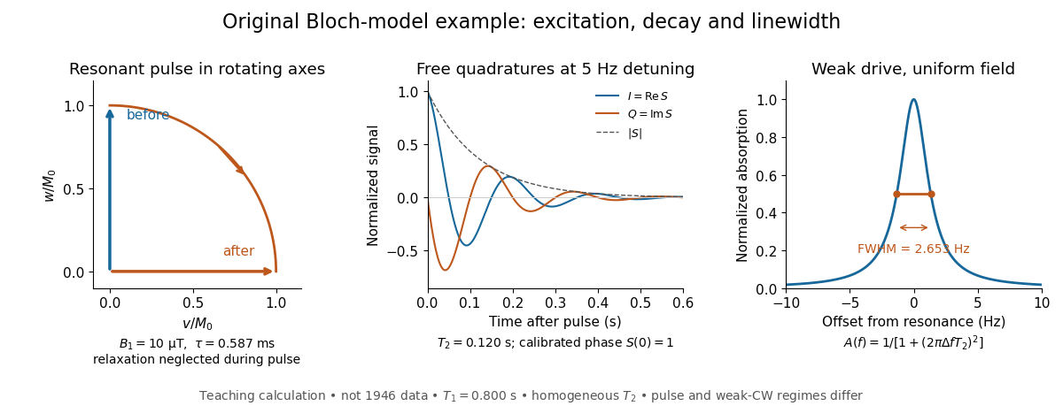
For constant drive, set the three rotating frame derivatives to zero. Substitution first gives , then , henceThe absorption is proportional to . With , its frequency dependence is a Cauchy distribution profile, often called a Lorentzian. With appreciable , the response broadens and on resonance: nuclear magnetic resonance saturation limits the response. The short-pulse amplitude in the previous example is not a weak continuous drive; these are different operating regimes of the same equations.
Drive reduces the longitudinal population imbalance when excitation competes with recovery. The dimensionless in the steady Bloch equations measures that competition.
For weak drive in this homogeneous model, half maximum occurs at . The absorption full width at half maximum is thereforeThe example gives or . At finite drive the model width is multiplied by . Field inhomogeneity and unresolved components can also broaden an actual line, so its width alone does not determine pure dephasing.
The same width appears by an original Fourier transform calculation. For and a free homogeneous signal demodulated exactly at resonance,This connects exponential memory to a Lorentzian absorptive line. It is a mathematical connection, not evidence that the 1946 teams performed pulsed Fourier transform spectroscopy. Instrumental signal bandwidth is a separate choice: narrowing a receiver band can reject thermal electrical noise, but too narrow a band distorts a changing signal. A sample linewidth and a receiver bandwidth are not interchangeable.
A spin echo is a reappearance of transverse magnetization after a pulse sequence reverses an earlier spread of phases. An ensemble can have almost no net transverse magnetization while its components retain enough individual phase memory to reassemble. In the ideal Hahn echo below, a short 90° pulse prepares transverse magnetization, a 180° pulse follows after time , and the signal refocuses at . The receiver observes freely precessing magnetization, as in free induction decay; no third driving pulse is needed at the echo time.
The useful distinction is between cancellation in an ensemble average and loss of recoverable phase memory. A static spread of Larmor precession frequencies can make free induction decay much faster than transverse nuclear magnetization decay. A spin echo can remove that static spread from the echo amplitude, allowing a more selective measurement of transverse relaxation. It does not in general reverse noise, population relaxation, or every interaction between spins.
Use the rotating frame and positive gyromagnetic ratio convention of free induction decay. Let be each component's fixed detuning, and normalize its magnetization by the equilibrium value. An instantaneous resonant pulse along rotates through about , preparing . A second pulse along rotates through about . These ideal pulses require a drive much stronger than the relevant detunings and negligible relaxation during either pulse. The corresponding rotation matrices, acting on column vectors, areHere is free Larmor precession in the rotating frame, before including transverse relaxation. Define a calibrated complex signal so the prepared component has . The pulse sends to its negative complex conjugate, hence sends to . Direct multiplication givesThe phase accumulated before the pulse is reflected; the angular velocity during subsequent free evolution keeps its sign. At every fixed detuning has zero residual phase. Equivalently, , so . This is not the identity on arbitrary three-dimensional magnetization: it returns the prepared component because . The two transverse pulse axes specified here also fix the receiver sign of the echo.
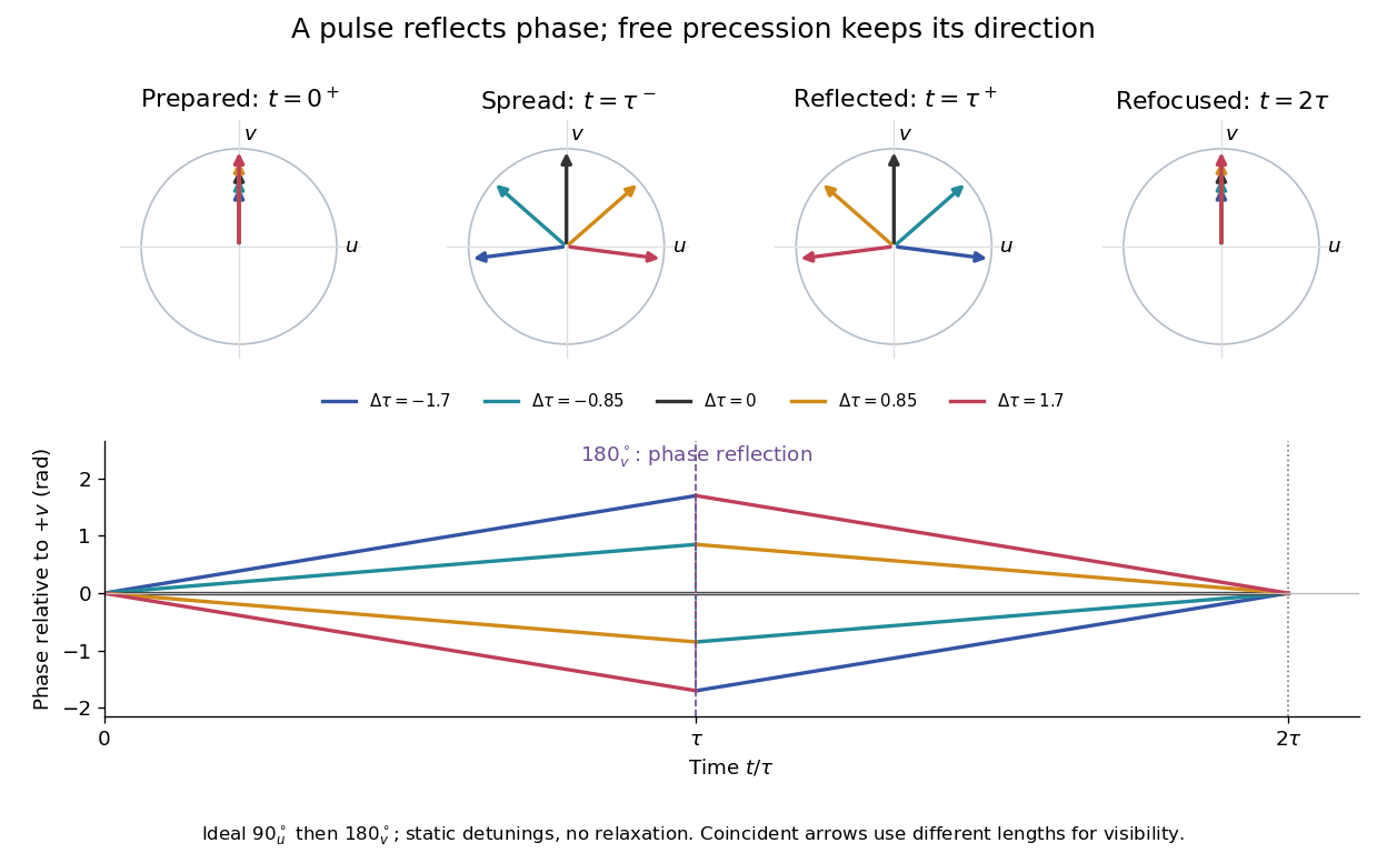
For an original ensemble example, let the static detunings have a Gaussian distribution with mean zero and standard deviation , independent of a common homogeneous . Averaging uses the characteristic function of that Gaussian distribution:Choose , and . Immediately before the refocusing pulse the normalized signal is only , yet . A one-pulse free induction decay at 80 ms would instead be about . These chosen numbers describe a calculation, not a measured trace. Increasing narrows the echo without changing in this ideal model. Because this Gaussian distribution produces a Gaussian factor rather than an exponential decay, its inhomogeneous decay is not characterized by a unique exponential .
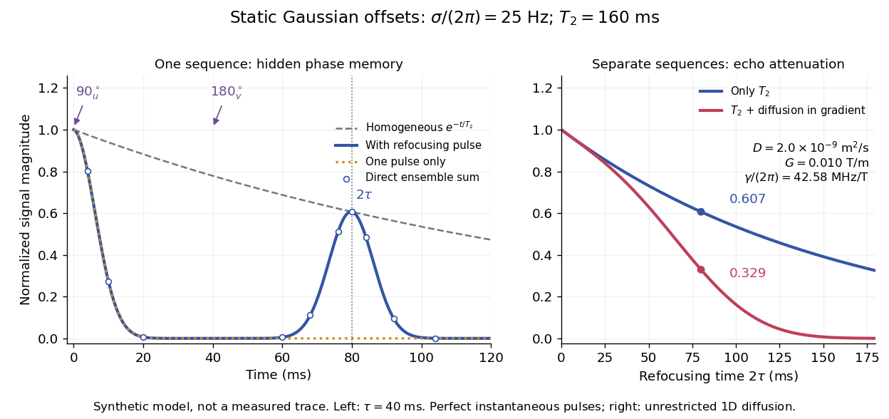
The exact phase-refocusing time is . A slowly falling transverse relaxation envelope moves the maximum of this particular echo shape slightly earlier: differentiating after the pulse gives , or here. Measuring consistently at avoids confusing this small envelope effect with a failure of refocusing. A series of such measurements gives only when the assumed homogeneous exponential decay, pulse quality and negligible additional attenuation are appropriate.
Erwin Louis Hahn's 1950 apparatus enclosed liquid samples in the coil of a tuned LC circuit, coupled to a gated radio transmitter and radio receiver. One transmitter quadrupled a crystal oscillator's 7.5 MHz to 30 MHz. A separate proton resonance regulator stabilized the static magnetic field.[ref]
Spin Echoes by Erwin Louis Hahn. §IV, Figs. 12–13: transmitter, coil, receiver and regulator
Waiting for thermal equilibrium prepared nuclear polarization. Oscilloscope photographs compared glycerol proton echoes at different field homogeneity: echo width changed; echo time followed twice the pulse separation. Receiver saturation obscured early free induction decay; transmitter leakage required care. The delayed signal tested refocusing; diffusion could still attenuate it.[ref]
Spin Echoes by Erwin Louis Hahn. §II(B), Fig. 2, §IV: preparation, timing, homogeneity comparison and readout limits
Hahn analyzed equal pulses as well as noting improved recovery with a second pulse twice as long; the ideal sequence above isolates that latter case.[ref]
A spin echo refocuses a nucleus's fixed detuning. A nucleus that moves through a magnetic field gradient can have different detunings during the two intervals. To see the distinction without assuming that all noise is reversible, let vary during free evolution. With the same pulse convention, its residual phase at isStatic detuning cancels because . A detuning during the first interval and during the second leaves , which need not vanish. The final component signal is before relaxation; changing the overall receiver convention changes its conjugation but not its magnitude.
For an original quantitative model, take a constant magnetic field gradient and unrestricted one-dimensional Brownian motion , where is the diffusion coefficient and is standard Brownian motion. Then . The constant terms cancel, and the Gaussian distribution of the remaining phase follows from the Brownian covariance kernel . Writing givesThe characteristic function of a zero-mean Gaussian distribution now supplies the extra factor , soHere is in radians per second per tesla, in tesla per metre, and in square metres per second: the extra exponent is dimensionless. The figure chooses , and . With the earlier and , diffusion reduces the echo from to about . These are illustrative model parameters, not values extracted from Hahn's experiment.
This result assumes instantaneous perfect pulses, a constant magnetic field gradient, unrestricted diffusion with constant diffusion coefficient, and independent homogeneous transverse relaxation. Restricted motion, changing gradients, finite pulses and interactions between spins can require different attenuation laws. Even a fixed Hamiltonian is refocused only for the terms whose sign the pulse reverses: a simultaneous 180° rotation of two spins leaves their product unchanged, because both factors change sign. A recovered echo therefore demonstrates a particular recoverable phase history, rather than reversal of every microscopic process.
Articles by others on the same topic

Nuclear Magnetic Resonance (NMR) is a physical phenomenon in which nuclei in a magnetic field absorb and re-emit electromagnetic radiation. This technique is primarily used to gain insights into the structure, dynamics, and environment of molecules in various fields, including chemistry, biochemistry, and medical imaging. ### Key Concepts of NMR: 1. **Nuclear Spins**: Certain atomic nuclei possess a property called spin, making them behave like tiny magnets.



Ciro Santilli once visited the chemistry department of a world leading university, and the chemists there were obsessed with NMR. They had small benchtop NMR machines. They had larger machines. They had a room full of huge machines. They had them in corridors and on desk tops. Chemists really love that stuff. More precisely, these are used for NMR spectroscopy, which helps identify what a sample is made of.
Introduction to NMR by Allery Chemistry
. Source. - only works with an odd number of nucleons
- apply strong magnetic field, this separates the energy of up and down spins. Most spins align with field.
- send radio waves into sample to make nucleons go to upper energy level. We can see that the energy difference is small since we are talking about radio waves, low frequency.
- when nucleon goes back down, it re-emits radio waves, and we detect that. TODO: how do we not get that confused with the input wave, which is presumably at the same frequency? It appears to send pulses, and then wait for the response.
How to Prepare and Run a NMR Sample by University of Bath (2017)
Source. This is a more direct howto, cool to see. Uses a Bruker Corporation 300. They have a robotic arm add-on. Shows spectrum on computer screen at the end. Shame no molecule identification after that!This video has the merit of showing real equipment usage, including sample preparation.
Says clearly that NMR is the most important way to identify organic compounds.
- youtu.be/uNM801B9Y84?t=41 lists some of the most common targets, including hydrogen and carbon-13
- youtu.be/uNM801B9Y84?t=124 ethanol example
- youtu.be/uNM801B9Y84?t=251 they use solvents where all protium is replaced by deuterium to not affect results. Genius.
- youtu.be/uNM801B9Y84?t=354 usually they do 16 radio wave pulses
NMR spectroscopy visualized by ScienceSketch
. Source. 2020. Decent explanation with animation. Could go into a bit more numbers, but OK.