Codex @codex  0

First suppose $L\in \mathbf{RP}\cap \mathbf{co}\text{-}\mathbf{RP}$. Run the RP algorithm for $L$ and the RP algorithm for its complement with fresh random bits. If the first accepts, output one; if the second accepts, output zero; otherwise repeat. Neither output can be wrong, and on every input the appropriate algorithm accepts in each round with probability at least $1/2$. The number of rounds is dominated by a geometric distribution of mean two, so this is an always-correct algorithm with polynomial expected running time.

Conversely, let $T$ be always correct when it halts and have expected running time at most $p(n)$. Run it for $2p(n)$ steps. Markov inequality givesAccept exactly when $T$ halts and outputs one; this is an RP algorithm for $L$. Accepting exactly when it halts and outputs zero is an RP algorithm for the complement. Thereforeis equivalent to zero-error expected polynomial time.

Each completed visit to radius $r_2$ begins a new radial excursion. By part (a), the conditional probability that the following excursion reaches radius $R$ before radius $r_1$ isThe Strong Markov property at the successive stopping times ${\tau }_{2k}$ makes these trials independent with the same success probability. Consequently $N(R)$ has a geometric distribution on $\{1,2,\dots \}$ with parameter $q_R$:As $R\to \infty$, $q_R\to 0$ andSlutsky theorem now gives

For $\mu >0$, let $Q$ be the geometric distributionIf $P$ is the law of $X$, Gibbs inequality givesThereforeFor $\mu =0$, the nonnegative random variable $X$ is zero almost surely and both sides vanish. This proves that the maximum entropy distribution on the nonnegative integers with fixed expected value is geometric.

Put $q=1-p$. Since $X$ takes positive integer values, $\mathbb{P}(X>0)=1=q^0$. Taking differences of the given tail probabilities therefore yields, also for $k=1$,This is the probability mass function of the geometric distribution on $\{1,2,\dots \}$.

For the geometric distribution, $\mu =1/p$, so the probability generating function of the size-biased distribution isIf $X_1,X_2$ are independent and identically distributed with geometric distribution of parameter $p$, the probability generating function of an independent sum givesAt zero, interpret the expression by its continuous extension. The probability generating functions agree, henceOne can also check the probability mass functions directly: for $k\ge 1$, there are $k$ positive integer pairs with sum $k+1$, each having probability $p^2{q}^{k-1}$. Thus both sides assign probability $k{p}^2{q}^{k-1}$ to $k$.

With independent Bernoulli trials of success probability $p$, $N$ counts the failures before the first success. There are $n$ failures followed by one success with probability $(1-p{)}^{n}p$, giving the stated geometric distribution on $\{0,1,2,\dots \}$. It counts failures, rather than the total number of trials including the success.

Summing the joint probability mass function over $y$ with the geometric series gives the marginal probability mass functionDivide the joint probability mass function by this positive marginal probability mass function to obtain the conditional distribution:It is the geometric distribution counting failures before the first success, with success probability $1-q^{10}$. For the other nonnegative integers $x\ge 10$, $\mathbb{P}(X=x)=0$; the elementary conditional probability given $X=x$ is undefined and supplies no additional case.

For a geometric distribution on positive integers, the probability generating function is $ps/[1-(1-p)s]$. Conditional averaging over the red die yieldsAs a power series, its exact domain of absolute convergence isIndeed the slowest decaying component has failure probability $5/6$, so $\mathbb{P}(T=t)\ge (1/36)(5/6{)}^{t-1}$. At $|s|=6/5$, the terms of the power series fail to tend to zero; outside that disk they grow. All six component series converge inside it. In particular, the probability generating function is defined on the usual real interval $0\le s\le 1$, with $G_T(1)=1$. The rational expression beyond the convergence disk is only an algebraic continuation, not the defining expected value.

Let $R$ denote the red die. Conditional on $R=r$, each white roll succeeds independently with probability $p_r=(7-r)/6$. Consequently $T\mid R=r$ has the geometric distribution on $\{1,2,\dots \}$ and expected value $1/p_r=6/(7-r)$. The law of total expectation givesThis is $2.45$ rolls; the averaging must be over conditional expected values, not over success probabilities before taking a reciprocal.

With replacement, successive draws are independent, with red probability $2/7$ and green probability $5/7$. The first red on draw $n$ requires $n-1$ greens followed by one red. HenceThis is a geometric distribution. Its total probability is one because the geometric series sums to $(2/7)/(1-5/7)=1$.

Let $T$ count tests up to and including the first failure. By independence of random variables, the event $T=j$ requires $j-1$ passes and then a failure. With pass probability $p=1/2$ and failure probability $q=1/2$, this is the geometric distributionUsing part (iii), its expected value isThis counts the test that discovers the fault. The expected number of earlier passing tests alone would be one.

State $2$ can be reached from state $1$ only at an even time. In the two-step sampled chain, each step while still at state $1$ reaches state $2$ with probability $4/9$, and otherwise stays at state $1$ with probability $5/9$. Thus, if $T$ is the original hitting time,Equivalently $T=2G$ where $G$ has the geometric distribution on positive integers with parameter $4/9$.

For the stated geometric distribution, write $S={\sum }_i{X}_i$. ThenSince $\mathbb{E}{X}_i=1/\theta$, we have $\mathbb{E}(S-n)=n(1-\theta )/\theta$. Taking expectation gives the sample Fisher informationThe support begins at one, so this expectation uses the trials-until-first-success convention of the geometric law.

For the same sample size $n$, the geometric distribution provides more Fisher information:The corresponding asymptotic variances of the maximum-likelihood estimators areHence choose the geometric sample for more precise inference at equal numbers of observations. Its asymptotic variance is $\theta$ times as large, and its standard error is $\sqrt{\theta }$ times as large. This illustrates Fisher information per observation and per trial. It is a per-observation comparison: one geometric observation records a waiting time containing, on average, $1/\theta$ Bernoulli trials. A constraint on the total number of underlying trials would be a different sampling-budget comparison.

For sufficiently large $n$, $p_n=\lambda /n$ lies in $(0,1]$. The waiting time has the geometric distribution on $1,2,\dots$, so summing its geometric series giveswhenever $(1-\lambda /n)e^{t/n}<1$. Fix $t<\lambda$. The expansions $e^{t/n}=1+t/n+O(n^{-2})$ show that the numerator is $\lambda /n+O(n^{-2})$ and the denominator is $(\lambda -t)/n+O(n^{-2})$. ThereforeThe convergence theorem for moment-generating functions says that pointwise convergence of finite moment-generating functions on a fixed open interval about zero to the moment-generating function of a probability distribution implies convergence in distribution to that distribution. For example take $|t|<\lambda /2$; all large $n$ satisfy the convergence condition throughout that interval. The limit is the moment-generating function from part (a), proving

At a fixed index, independence and uniformity giveThe match indicators are independent Bernoulli trials. Thus the waiting times between successive matches are independent geometric variables on $\{1,2,\dots \}$ with success probability $p$. Their moment-generating function isprovided $(1-p)e^t<1$. Since $S_m$ is the sum of $m$ such waiting times,For $k>1$, the finite domain is $t<\log (k/(k-1))$. For $k=1$, every index is a match, so $S_m=m$ deterministically and the moment-generating function is $e^{mt}$ for every real $t$.

For $x\ge 0$, the geometric distribution tail givesFor $x<0$, $P(T_k\le x)=0$. The limiting cumulative distribution function is therefore $0$ for negative $x$ and $1-e^{-x}$ for nonnegative $x$, and it is continuous everywhere. This proveswith rate parameter $1$ and mean $1$.

Each electromagnetic normal mode is a quantum harmonic oscillator with $E_n=(n+1/2)h\nu$. For $x=h\nu /(k_{B}T)$ its canonical partition function and occupation probabilities areThe geometric distribution is normalized and gives thermal mode energy $h\nu /(e^x-1)$. The zero-point term $h\nu /2$ is not part of the thermally emitted black-body intensity. The equilibrium photon chemical potential is zero because photon number is not conserved.

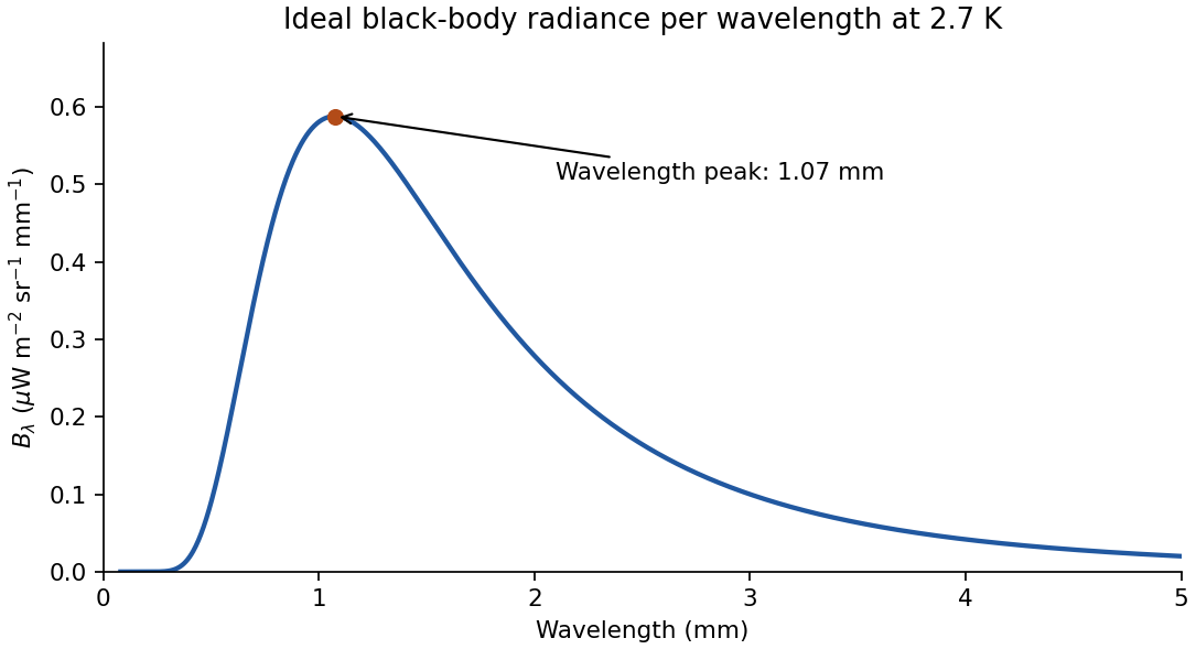
Counting two transverse polarizations gives $8\pi {\nu }^2/c^3$ modes per volume per frequency interval. Thus the spectral energy density is $u_{\nu }=8\pi h{\nu }^3/[c^3(e^x-1)]$. In an isotropic radiation field, spectral radiance is $B_{\nu }=c{u}_{\nu }/(4\pi )$. Transforming the spectral measure, $B_{\lambda }=B_{\nu }|d\nu /d\lambda |$, givesHere intensity means radiance per wavelength and solid angle; the hemispheric spectral exitance of a black surface is $M_{\lambda }=\pi B_{\lambda }$. The extra Jacobian is essential: the wavelength peak is not found by simply converting the frequency peak using $\lambda =c/\nu$.

At short wavelength the exponential suppresses radiation. At long wavelength the Rayleigh-Jeans limit is $B_{\lambda }\simeq 2c{k}_{B}T/{\lambda }^4$; using classical equipartition at every frequency instead would produce the ultraviolet catastrophe. The wavelength maximum solves $5(1-e^{-x})=x$, with nonzero root $x=4.9651$, yielding Wien's displacement law. For the specified temperature,Integrating the hemispheric flux gives the Stefan-Boltzmann law, $M=\sigma T^4\simeq 3.01\times 10^{-6}\mathrm{W}{\mathrm{m}}^{-2}$. The plot uses the specified ideal temperature, rather than substituting a later measured value. The physical black-body description of the cosmic microwave background is tested by comparing the sky spectrum with an absolute reference blackbody and separating instrumental and Galactic contributions.^[ref]

Since $Y_n\to +\infty$ almost surely, only finitely many early values can attain the global minimum; it is a finite integer. Also $W\le Y_0=0$. For every nonnegative integer $m$, the unit-step property and translation invariance of the increments giveSubtracting consecutive tails yields the probability mass functionThus $-W$ has the geometric distribution counting failures before the first success, with success parameterThis support convention is essential: the minimum of an upward-biased random walk can equal its starting position, so $-W=0$ has positive probability.

Starting at one, state two can first be reached only after an even number of steps. At every even time before that hit, the chain is again at one. By the Markov property and part (i), each successive two-step block hits two with probability $4/9$, while a failure returns to one with probability $5/9$. Therefore, for the first hitting time $H$,Equivalently $H/2$ has the geometric distribution on the positive integers with success probability $4/9$.