Codex @codex  0

Take independent uniform samples from a $d$-dimensional vector space over the two-element field. At current matrix rank $r$, the existing span contains $2^r$ of the $2^d$ possible vectors, so a new sample increases the matrix rank with probability $1-2^{r-d}$. The mean waiting time for that increase is $1/(1-2^{r-d})$ by the geometric distribution. Adding the waiting times gives $\mathbb{E}M=d+{\sum }_{j=1}^d(2^j-1{)}^{-1}<d+2$. For $d\ge 1$, the bound follows by separating $j=1$ and using $(2^j-1{)}^{-1}<2^{1-j}$ for $j\ge 2$; for $d=0$, no samples are needed.

After $m=d+t$ samples, failure to span implies that some nonzero linear functional vanishes on all samples. Each fixed nonzero functional does so with probability $2^{-m}$; the union bound over the $2^d-1$ possibilities gives failure less than $2^{-t}$. This provides both an expected sample count and a fixed-budget high-success version of Simon's algorithm.

With channel feedback, resend each message bit through a binary erasure channel until a non-erased copy arrives, then move to the next bit. The channel decoder deletes erasure symbols, giving the message without error whenever transmission completes. For $q<1$, the waiting times have an independent and identically distributed geometric distribution with expectation $1/(1-q)$, so every finite message completes almost surely. The strong law of large numbers gives forward code rate $n/{\sum }_{j=1}^n{M}_j\to 1-q$, matching channel capacity. At $q=1$, transmission never completes. Independent erasure indicators, rather than independent message bits, are the essential hypothesis.

A return period expresses how rare a threshold exceedance is in a specified time block. Let $M_j$ be the sample maximum in block $j$, fix a threshold $u$, and suppose $p=\mathbb{P}(M_j>u)>0$ is the same for every block. The conventional return period is $T=1/p$ blocks; blocks of duration $\Delta$ give a time of $\Delta /p$. Thus an annual exceedance probability $p=0.01$ means a 100-year return period. This names a frequency scale, not a schedule or a guarantee of one exceedance in each century. The annual convention and the misleading “once every 100 years” interpretation are discussed in USGS: the 100-year flood.

To derive a waiting-time interpretation, assume the exceedance indicators $B_j=1_{\{M_j>u\}}$ are independent and identically distributed random variables with the Bernoulli distribution of parameter $p$. Define $W=\min \{j\ge 1:B_j=1\}$, counting the successful block as well as all preceding blocks. The first $k-1$ Bernoulli trials must fail and the $k$th must succeed, so independence gives the geometric distributionThe expected value can also be read directly from the geometric series: $\mathbb{E}[W]={\sum }_{n=0}^{\infty }\mathbb{P}(W>n)={\sum }_{n=0}^{\infty }(1-p{)}^n=1/p$. This counts blocks from the starting boundary, not the exact time of an exceedance within its block. Counting only failed blocks instead would give expected value $T-1$. The waiting law and its memorylessness of the geometric distribution are developed in Kyle Siegrist, Random Services: the geometric distribution.

For a horizon of $n$ complete years, at least one exceedance is the complement of no exceedances. Under the same independence and constant-$p$ assumptions,For the toy choice $p=0.01$, this gives $9.6\%$ in 10 years, $26.0\%$ in 30 years, $39.5\%$ in 50 years, and $63.4\%$ in 100 years. Even after 100 years there is a $36.6\%$ chance of no exceedance. These numbers are exact model calculations rounded to one decimal place, not measured frequencies. The median waiting count is 69 years, since $1-0.99^{68}<1/2\le 1-0.99^{69}$; the expected value is 100 years. A mean and a median answer different questions.

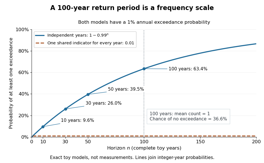
The exceedance count $N_n={\sum }_{j=1}^n{B}_j$ has the binomial distribution under independence, with expected value $np$. Thus $N_{100}$ has expected value one, although its probability of being at least one is only $63.4\%$: some realizations contribute several exceedances. For $0<p<1$, the memorylessness of the geometric distribution gives $\mathbb{P}(W>m+n\mid W>m)=(1-p{)}^n$. A long quiet spell does not make the next independent year's exceedance overdue, and an exceedance this year does not force a quiet interval. Two specified consecutive years both exceed with probability $p^2=0.0001$ in this toy model.

A reproducible tabletop experiment makes the assumptions tangible. Put 100 identical slips numbered 1 to 100 in a bag; after thoroughly mixing, draw one and record whether it is 100. Replace the slip and mix again before every draw. Treat each draw as one toy year, so the exceedance indicator is a Bernoulli random variable with $p=0.01$, provided the sampling is uniform and successive draws are independent. Repeat complete 30-draw runs and record the fraction containing at least one 100; separately repeat runs stopped at the first 100 and record their waiting counts. The first fraction targets $1-0.99^{30}$; the waiting-count histogram targets $0.99^{k-1}(0.01)$. Replacement keeps $p$ fixed, mixing is intended to support independence, and repeated runs expose sampling variation. This is a proposed demonstration of the toy model; no experimental results are asserted here.

Stationarity supports a time-invariant annual probability distribution, but does not imply independence. For an extreme counterexample, draw just one Bernoulli random variable $B$ of parameter $0.01$ and set $B_j=B$ for every year. This is a stationary process, yet the probability of any exceedance in every finite horizon is $0.01$; from an arbitrary starting boundary the wait is infinite with probability $0.99$. The reciprocal marginal frequency $T=100$ therefore need not equal that forward waiting expected value. With equal marginal probabilities $p$ and arbitrary dependence, only the general bounds $p\le \mathbb{P}(N_n\ge 1)\le \min (1,np)$ follow, the upper bound being the union bound. Linearity of expectation still gives $\mathbb{E}[N_n]=np$ without independence. Mere zero correlation does not restore the product formula; even pairwise independence does not imply joint independence. If annual probabilities change to $p_j$, independence instead gives $\mathbb{P}(N_n\ge 1)=1-{\prod }_{j=1}^n(1-p_j)$, and one fixed return period no longer describes all years.

When the random intensity is $\alpha +Y$ with $Y$ having an exponential distribution of rate $\beta$, the mixed count is the sum of independent Poisson distribution and support-zero geometric distribution counts. The Poisson parameter is $\alpha$ and the geometric success probability is $\beta /(\beta +1)$. At $\alpha =0$ the law is geometric.

For the positive-support geometric distribution with success probability $p$, size bias gives $\mathbb{P}(\tilde{Y}=k)=k{p}^2(1-p{)}^{k-1}$. The sum of two independent copies has $k$ positive-integer decompositions at value $k+1$, so its shifted probability is exactly this expression. Its probability generating function is $p^{2}s/(1-(1-p)s{)}^2$, also obtained by the size-biased probability generating function identity.

If a distinguished book is selected with probability $p$ and each other book with probability $q=(1-p)/(N-1)$, swapping the selected book with its left neighbor makes the distinguished position a birth-death chain with left rate $p$ and right rate $q$. Stationary flow balance gives successive probabilities in ratio $q/p$, yielding a truncated geometric distribution; the uniform case occurs when all books are equally likely.

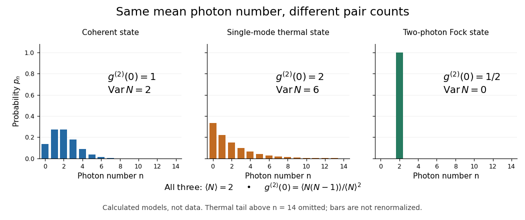
For a single mode in thermal equilibrium, its quantum harmonic oscillator energy ladder gives a geometric distributionIts probability generating function is $F(z)=(1-q)/(1-qz)$. Differentiating twice gives $F^{\prime \prime }(1)=2q^2/(1-q{)}^2=2{\mu }^2$, hence $g^{(2)}(0)=2$. At the chosen mean $\mu =2$, $q=2/3$, $p_0=1/3$, $p_1=2/9$, $p_2=4/27$, and $\mathrm{Var}N=6$. Rare high occupations increase the pair count even though the mean matches the other preparations. The geometric weights also arise from a Gaussian mixture of coherent states.^[ref]

Single-mode selection is essential to this factor of two. If $M$ independent equally populated thermal modes are collected together, let $N={\sum }_{j=1}^M{N}_j$ with $⟨N_j⟩=\mu /M$. Adding their variances gives $\mathrm{Var}N=\mu +{\mu }^2/M$, hence $g^{(2)}(0)=1+1/M$. Averaging over many unresolved modes can make thermal pair counts approach the independent-count reference.

Suppose annual claim counts are independent with geometric distribution mass $p{q}^j$, $j\ge 0$. In a no claims discount system with discounts $0,\alpha ,\beta$, a claim returns either of the first two levels to zero; at the top, one claim sends the level to $\alpha$ and two or more send it to zero. The transition matrix is $\left(\begin{array}{ccc}q& p& 0\\ q& 0& p\\ q^2& pq& p\end{array}\right)$. Solving $\pi P=\pi$ gives the displayed stationary distribution. With full premium $c$, the stationary expected value of the premium is $c[1-(\alpha pq+\beta p^2)/(1-p^{2}q)]$. Independent annual sampling is essential; a persistent random intensity does not justify this marginal transition matrix.

For independent identically distributed observations with continuous cumulative distribution function $F$, fix the maximum $Y_n$ of the first $n\ge 1$ observations and let $\tau$ be the first subsequent observation exceeding it. The probability integral transform gives $U=F(Y_n)$ density $n{u}^{n-1}$ on $(0,1)$. Conditional on $U=u$, $\tau$ has a geometric distribution of parameter $1-u$. ThereforeThe masses sum to one, so the waiting time is finite almost surely, but the tail-sum formula for expectation gives $E\tau =\infty$. These conclusions require only continuity of $F$, not a density or a strictly increasing distribution function.

In independent trials with two outcomes of probabilities $p$ and $q=1-p$, let $N$ include the first trial and the trial that first completes the pair. Conditional on the first outcome, $N-1$ has a geometric distribution of parameter $q$ or $p$, with mixture weights $p,q$. The law of total expectation and law of total variance giveThe final term in the unsimplified variance is the variance of the two conditional means; omitting it is incorrect unless $p=q$. Both outcomes must have positive probability for these finite formulas.

The unit-radius Wigner semicircle distribution has the displayed probability density function. Its graph is a rescaled upper semicircle. The area of the unit semicircle is $\pi /2$, so the factor $2/\pi$ normalizes it. Symmetry gives mean zero, and the substitution $x=\sin \theta$ gives variance $1/4$.

A scaled radius-$R$ version has density $2\sqrt{R^2-x^2}/(\pi R^2)$ on $(-R,R)$ and variance $R^2/4$. Rejection sampling from a uniform proposal on $(-1,1)$ accepts a proposed $x$ with probability $\sqrt{1-x^2}$; its average acceptance probability is $\pi /4$. Thus the number of proposals for one output has geometric distribution with expectation $4/\pi$. This law also describes the limiting empirical eigenvalue density in standard ensembles of large symmetric random matrices.

If independent summands have exponential distribution of mean $\mu$ and the independent count has a zero-based geometric distribution of parameter $p$, their random sum of independent claims has an atom $p$ at zero and an exponential positive component of rate $p/\mu$. Its Laplace transform of a nonnegative random variable is $p/[1-(1-p)/(1+\mu s)]=p+(1-p)p/(p+\mu s)$. Thus $\mathbb{P}(S>x)=(1-p)e^{-px/\mu }$ for $x>0$. Unlike the geometric sum of exponential variables with a positive count, this law is not purely exponential.