Hazard function ($h(t)$)

For a survival time with an absolutely continuous probability distribution, probability density function $f$, and survival function $S$, the hazard function iswhere $S(t)>0$, with the derivative identity holding almost everywhere. At points where the local limit exists, equivalentlyThe hazard function measures an instantaneous conditional rate. If time is in years, its units are inverse years, and its value can exceed one. A probability for a short interval is approximately $h(t)\Delta$, not $h(t)$; for an absolutely continuous probability distribution, the probability of an occurrence at the single exact time $t$ is zero. The discrete hazard, by contrast, is a conditional probability at a possible event time.

The factorization $f(t)=h(t)S(t)$ distinguishes a probability density function for the original population from a hazard function for those still event-free. With an exponential distribution of rate $0.2$ per year, $h(5)=0.2$ per year but $f(5)=0.2e^{-1}\approx 0.073576$ per year: the latter also accounts for the probability of reaching year five. The exponential survival risk over an interval example computes finite-horizon probabilities from this rate.

Upper records of iid observations with a continuous distribution have transition density $f(w)/(1-F(v))$ above the latest record $v$. Consequently the cumulative hazard $\Lambda (v)=-\log (1-F(v))$ transforms consecutive record increments into independent unit exponentials. Record counts below a level $t$ with $F(t)<1$ are therefore Poisson with mean $\Lambda (t)$. Set the count to zero if the first record exceeds the level. At a finite upper endpoint with $F(t)=1$, the count is infinite instead of a finite-mean Poisson variable.

At ordered possible failure times $t_j$, the discrete hazard is $h_j=\mathbb{P}(T=t_j\mid T>t_{j-1})$. Its survival function satisfies $S(t_j)=S(t_{j-1})(1-h_j)$, and hence $S(t)={\prod }_{t_j\le t}(1-h_j)$. Estimating $h_j$ by the observed number of failures divided by the risk set size under independent censoring yields the Kaplan–Meier estimator. Unlike a continuous-time hazard rate, a discrete hazard is a probability between zero and one.

For an equally weighted mixture of individual survivor functions $F_i$, the population hazard function is $\overline{h}(t)={\sum }_i{F}_i(t)h_i(t)/{\sum }_i{F}_i(t)$. Thus the weights are the surviving proportions, and the cumulative hazard function is $-\log (n^{-1}{\sum }_i{e}^{-H_i(t)})$, not generally the mean individual integrated hazard.

For a nonnegative random constant individual hazard $\Lambda$, write $M_k(t)=\mathbb{E}[{\Lambda }^k{e}^{-\Lambda t}]$. The population survivor function is $M_0$ and its hazard is $M_1/M_0$. Under the integrability needed to differentiate, $M_k^{\prime }=-M_{k+1}$, soThe conditional distribution is weighted by $e^{-\Lambda t}$. This proves decreasing population hazard without any decrease in individual hazards and explains survival selection in a heterogeneous population.

In a population mixture with initial component probabilities $p_i$, conditioning on survival to time $t$ changes them to the displayed probabilities by Bayes' theorem. Components with larger survivor functions receive greater relative weight among survivors. The population hazard function is the weighted mean of the component hazards with these time-dependent weights. This selection can change the population hazard even when all component hazards are constant, as shown by the hazard derivative for a mixture of exponential distributions.

For a finite mixture with positive weights $p_i$ and rates ${\lambda }_i>0$, the survivor function is $S(t)={\sum }_i{p}_i{e}^{-{\lambda }_{i}t}$ and the hazard function is the surviving-population mean of the component rates. Write $w_i(t)=p_i{e}^{-{\lambda }_{i}t}/S(t)$. Differentiation gives $w_i^{\prime }=w_i(h-{\lambda }_i)$ and therefore $h^{\prime }=h^2-{\sum }_i{w}_i{\lambda }_i^2=-\mathrm{Var}(\Lambda \mid T>t)$. The hazard is decreasing, strictly so when distinct rates have positive weights. For finitely many rates it tends to the smallest rate with positive weight. This is survival selection even though each individual component has a constant hazard.

Suppose $T\ge 0$ has an absolutely continuous probability distribution, with survival function $S(0)=1$. On an interval where $S(t)>0$, its cumulative hazard isHere $h$ is the hazard function; its integral is dimensionless because the units of rate and time cancel. The identity follows by integrating the derivative of $\log S$, so mere continuity of the survival function is not enough: the absolute continuity assumption supplies a probability density function. If $S$ reaches zero, interpret $-\log S$ as $+\infty$. The normalization $S(0)=1$ also matters; an initial probability mass at zero would require an initial term $-\log S(0)$.

Accumulating hazard functions adds on the $H$ scale and multiplies survival factors on the $S$ scale. For $S(a)>0$ and $b>a$,For instance, a cumulative hazard increment of $2$ gives event probability $1-e^{-2}\approx 0.864665$, rather than a probability of $2$. With $h(t)=0.2$ per year, $H(5)=1$ and $S(5)=e^{-1}\approx 0.367879$. With the increasing hazard function $h(t)=0.04t$ per year when $t$ is expressed in years, $H(t)=0.02t^2$, so $H(5)=0.5$ gives $S(5)=e^{-0.5}\approx 0.606531$. Its coefficient has units of inverse years squared.

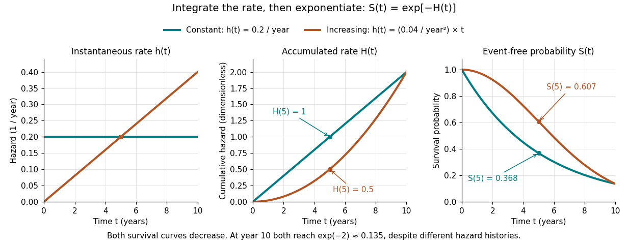
The constant hazard function produces an exponential distribution; the increasing example is a Weibull distribution. Their survival functions both decrease, although one hazard function stays constant and the other increases. At year ten both have $H(10)=2$ and $S(10)=e^{-2}$ despite different earlier histories. The accumulation identity is described in Lu Tian's Stanford notes, Section 1.1.

For a discrete hazard $q_j$ at each possible event time $t_j$, the exact counterpart is $S(t)={\prod }_{t_j\le t}(1-q_j)$. Taking its negative logarithm sums $-\log (1-q_j)$, rather than $q_j$. Therefore exponentiating a Nelson–Aalen estimator does not give exactly the Kaplan–Meier estimator; small-jump comparison of cumulative hazard estimators quantifies the difference.

Let $X=\min (T,C)$, $V=1_{\{T\le C\}}$, and suppose $T$ and $C$ are independent, with continuous failure density $f=hS$. Then the Tonelli theorem givesThus $V-H(X)$ has mean zero. The identity also holds conditionally on covariates when censoring is independent conditionally on them. For an estimated hazard, the mean error is controlled by $\mathbb{E}|\hat{H}(X)-H(X)|$, not by pointwise fit alone.

// Target: survival-analysis.bigb

For a nonnegative continuous event time with survival function S, hazard function h and H the cumulative hazard, split the expectation at c. The censored contribution is S(c)H(c). The event contribution is ${\int }_0^{c}H(t)f(t)dt=1-S(c)-S(c)H(c)$ by integration by parts, since $dH=hdt$ and $f=hS$. Adding gives the displayed identity. Linearity extends it to the expected observed event count in a cohort, without requiring independence between subjects.

For a proper continuous event time and invertible cumulative hazard function $H$, the survivor function identity $F(t)=e^{-H(t)}$ gives $H(T)\sim \mathrm{Exp}(1)$.

A hazard ratio compares two hazard functions at the same time. Under proportional hazards it is constant in time.