Codex @codex  0

Equip the symmetric group $S_n$ with its uniform probability measure and unnormalized Hamming distance. If $f$ has Lipschitz constant $K$, it obeys the displayed two-sided bound, and each one-sided tail has the same exponential without the factor two. Reveal a uniform permutation one image at a time. Two possible next images have completion sets paired by swapping those two values, changing exactly two coordinates. Thus the corresponding conditional means differ by at most $2K$. Each increment of the Doob exposure martingale has conditional range length at most $2K$. Applying the conditional Hoeffding lemma gives $\mathbb{E}{e}^{\lambda (f-\mathbb{E}f)}\le e^{n{\lambda }^2{K}^2/2}$; optimizing the exponential Markov bound proves the bound. A mere absolute-increment bound of $2K$ gives a weaker constant, so using the range length matters.

Expose independent coordinates successively and take the conditional mean of a function after each exposure. These conditional means form a martingale from $\mathbb{E}f$ to $f$. A coordinate oscillation bound $c_i$ gives a conditional interval of length $c_i$ for the corresponding increment, by coupling the unexposed coordinates. Applying the Hoeffding lemma to these conditional ranges proves the McDiarmid inequality.

The Hoeffding inequality turns finite interval bounds and independence into exponentially small tail probabilities for a sum. It requires neither a normal distribution nor identical probability distributions. Let $X_1,\dots ,X_n$ be independent essentially bounded real random variables, with deterministic finite bounds $a_i\le X_i\le b_i$ almost surely. Define the centered sum and its squared-width budget byFor $V>0$ and $t>0$,The union bound therefore gives $\mathbb{P}(|S_n|\ge t)\le \min \{1,2e^{-2t^2/V}\}$. If $V=0$, every $X_i$ is constant almost surely, so $S_n=0$ and both positive-threshold tail probabilities vanish. The equal-width version is stated in the authored Stanford notes.^[ref]

The quantity $V$ is a sum of squared interval widths, not the variance of $S_n$. Centering changes the endpoints to $a_i-\mathbb{E}{X}_i$ and $b_i-\mathbb{E}{X}_i$, leaving each width unchanged. For example, independent random variables in $[-2,1]$ and $[4,5]$ have $V=3^2+1^2=10$, whatever their expected values or probability distributions. A deviation at least three above their total expected value has probability at most $e^{-18/10}\approx 0.165299$. If all widths equal $b-a>0$, the sample mean ${\overline{X}}_n=n^{-1}{\sum }_i{X}_i$ satisfies

Independence is essential to this general guarantee. Take one Bernoulli random variable $B$ with success probability $1/2$ and set every $X_i=B$. Each lies in $[0,1]$, but for every $n$ the sample mean is either zero or one. Thus $\mathbb{P}(|{\overline{X}}_n-1/2|\ge 1/4)=1$, whereas incorrectly inserting these dependent observations into the formula would give $2e^{-n/8}$, less than one for $n\ge 6$. Some special dependent models have their own valid concentration inequalities; arbitrary statistical dependence cannot be ignored.

For the short proof, apply Markov's inequality to $e^{\lambda S_n}$ with $\lambda >0$, factor the expectation using independence, and apply the Hoeffding lemma to each factor:Minimizing this quadratic polynomial at $\lambda =4t/V$ gives the upper tail probability; applying it to $-S_n$ gives the lower one. This is the Chernoff bound method. The original 1963 article is Probability Inequalities for Sums of Bounded Random Variables by Wassily Hoeffding; its publisher record identifies the article, but its full text was unavailable during this source check. The argument above is a direct derivation rather than a claim to have inspected that article's proof.

The Hoeffding lemma controls the entire centered moment-generating function using only an interval width. For an essentially bounded real random variable $X$ with finite deterministic bounds $a\le X\le b$ almost surely, every real $\lambda$ satisfiesEquivalently, $\mathbb{E}{e}^{\lambda (X-\mathbb{E}X)}\le e^{{\lambda }^2(b-a{)}^2/8}$. This single-random variable statement needs no independence assumption; independence enters when applying it to the factors for a sum in the Hoeffding inequality. Both signs of $\lambda$ are allowed, and equality holds at $\lambda =0$ or when $a=b$.^[ref]

In the convention $\log \mathbb{E}{e}^{\lambda Y}\le {\lambda }^2{\sigma }^2/2$ for a centered sub-Gaussian random variable $Y$, the Hoeffding lemma supplies ${\sigma }^2=(b-a{)}^2/4$. This upper parameter need not equal the actual variance. For a Bernoulli random variable $B$ of success probability $p$,The actual variance is $p(1-p)$, whereas the supplied parameter is $1/4$ for every $p$. This explains part of the conservatism visible in Hoeffding sample size for Bernoulli frequencies.

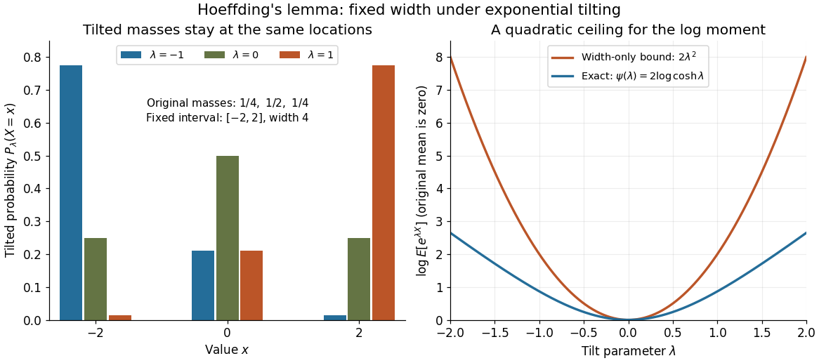
A short proof exposes why the constant is $1/8$. Put $Y=X-\mathbb{E}X$ and define exponential tilting byThe tilted probability measure has the same interval of possible values, and differentiating the cumulant-generating function gives ${\psi }^{\prime \prime }(\lambda )={\mathrm{Var}}_{{\mathbb{P}}_{\lambda }}(Y)$. Boundedness justifies these derivatives for every finite $\lambda$. Under any such tilted law, Popoviciu's inequality on variances gives ${\psi }^{\prime \prime }(\lambda )\le (b-a{)}^2/4$: the variance is no larger than the expected value of the squared distance from the interval midpoint, itself at most $(b-a{)}^2/4$. Since $\psi (0)={\psi }^{\prime }(0)=0$, the integral form of Taylor's theorem yieldsThis expression handles either sign of $\lambda$ without changing the argument.

The constant $1/8$ cannot be reduced uniformly over all essentially bounded real random variables. Equal endpoint probabilities at $a$ and $b$ give $Y=\pm (b-a)/2$, a scaled Rademacher random variable, andThus the sharpness is already forced near zero by the variance; the bound need not be equality at nonzero parameters for a particular probability distribution.

Let $(A_t,B_t)$ be a Markov jump process on integer populations, with rateswhen $a,b>0$, where $\kappa >0$. Make both axes absorbing, so the fight ends when one population reaches zero. Start at $(N,b_N)$, with $b_N=\lfloor \alpha N\rfloor$; when $\alpha N$ is integral this is the printed initial condition exactly. The harmless rounding convention makes the model defined for every integer $N$.

Use the embedded jump chain $(A_j,B_j)$ rather than physical time. Its probabilities of the two losses are respectively $b/(a+b)$ and $a/(a+b)$, independently of $\kappa$. It reaches an axis after at most $N+b_N\le 2N$ steps; hold it constant thereafter. PutBefore absorption its two increments are $-2a+1$ and $2b-1$, soAfter absorption set ${\mu }_j=0$. Consequentlyis a discrete-time martingale. All populations are at most $N$, so each martingale difference is bounded in absolute value by $2N+2\le 4N$. The total drift up to step $2N$ is at most $2N$. This is the squared-population near-invariant for stochastic attrition.

The two-sided Azuma-Hoeffding inequality states that a martingale with $m$ differences bounded by $C$ satisfies $\mathbb{P}(|M_m|\ge z)\le 2\exp (-z^2/(2m{C}^2))$. Its exponential estimate follows by applying the conditional Hoeffding lemma to each centered difference, iterating, and optimizing the exponential Markov bound. With $m=2N$ and $C=4N$ it gives

Let $c=\sqrt{1-{\alpha }^2}>0$, and let $X^N=A_{2N}/N$ be the final proportion. If the first population survives, then the second is zero and $D_{2N}/N^2=(X^N{)}^2$. Hence $|X^N-c|>\delta$ impliesIf the first population is extinguished, $X^N=0$ and $D_{2N}\le 0$. This can satisfy the indicated deviation event only when $\delta <c$, and then $|D_{2N}-c^2{N}^2|\ge c^2{N}^2>c\delta N^2$. Thus the same implication holds in both cases.

The initial rounding error obeys $|D_0-c^2{N}^2|=|{\alpha }^2{N}^2-b_N^2|\le 2N$. Combining it with the drift bound shows that the deviation event forcesfor all sufficiently large $N$. Set $\eta =c\delta /2$ in the preceding concentration inequality. We concludefor sufficiently large $N$, and thereforeThe symmetric stochastic attrition process thus has exponential concentration of terminal stochastic attrition survivors. The deterministic equations conserve $a^2-b^2$ and predict the same surviving fraction, but the martingale argument supplies the stronger exponential probability estimate required here.

Expose the independent coordinates in order and let $M_i=\mathbb{E}[f\mid X_1,\dots ,X_i]$, $M_0=\mathbb{E}f$. This is the Doob exposure martingale. For fixed earlier coordinates, write $h_i(x)=\mathbb{E}[f\mid X_i=x,\text{earlier coordinates}]$. The remaining coordinates have the same distribution for all $x$, and the coordinate-change hypothesis gives $|h_i(x)-h_i(y)|\le c_i$. Thus the conditional range of $M_i-M_{i-1}$ has length at most $c_i$, and its conditional mean is zero.

Here is the Hoeffding lemma needed for the sharp constant. If a mean-zero random variable $Y$ lies in an interval of length $c$, set $\psi (s)=\log \mathbb{E}{e}^{sY}$. Its second derivative is the variance under the exponentially tilted law. Under any such law, variance is at most $c^2/4$, by comparison with squared distance from the interval midpoint. Since $\psi (0)={\psi }^{\prime }(0)=0$, integration gives $\psi (s)\le s^2{c}^2/8$ for all real $s$. Applying this conditionally and iterating the tower property yieldsThe exponential Markov bound now givesFor $C>0$ choose $s=4t/C$. Apply the same argument to $-f$ and add the two tails, proving the McDiarmid inequalityFor $C=0$, $f$ is constant almost surely, and every positive-deviation probability is zero.

For the neighbourhood application, the ambient points must be elements of $\mathcal{P}[n]$, equivalently binary strings; the printed $y\in [n]$ is a type error. An $n$-element ambient set could not generally satisfy the stated exponential-size lower bound. Use the uniform product probability space on the Boolean cube and set $F(y)=d(y,A)$. Flipping one coordinate changes this Hamming distance by at most one, so $C=n$. Put $\mu =\mathbb{E}F$. Since $\mathrm{Pr}(F=0)=|A|/2^n\ge \epsilon$, the proved two-sided inequality gives, for $\mu >0$,Consequently $\mu \le \sqrt{(n/2)\log (2/\epsilon )}=t/2$; the same bound is immediate if $\mu =0$. ThereforeThis proves the Boolean cube expansion from bounded differences:The meaningful range is $0<\epsilon \le 1$; real radii are interpreted by the inequality on the integer-valued Hamming distance. The converted TeX's final $2^{2n}$ is another corruption: the original PDF has $2^n$.

The exponent printed in the original PDF is too strong under the stated increment bound. Take $M_0=0$, let $M_1$ equal $1$ or $-1$ with equal probabilities, and set $M_k=M_1$ for $k\ge 1$. This is a martingale with $c_1=1$ and $c_k=0$ for $k>1$. For $n=1$ and $x=1$,Thus the printed inequality is false. The intended two-sided Azuma-Hoeffding inequality isHere the $c_k$ are deterministic increment bounds. We prove this corrected assertion from conditional exponential moments.

Let $D_k=M_k-M_{k-1}$. The martingale property gives $\mathbb{E}[D_k\mid {\mathcal{F}}_{k-1}]=0$. For $c_k>0$, convexity of the exponential function gives the secant bound on $[-c_k,c_k]$,Taking conditional expectation removes the terms containing $D_k$, soThe last inequality follows term by term from $(2j)!\ge 2^{j}j!$ in the power series for $\cosh z$ and $e^{z^2/2}$. If $c_k=0$ the increment is zero and the same bound holds directly. This is the bounded-increment case of the Hoeffding lemma.

Repeated conditioning, without any independence assumption, now givesWrite $C={\sum }_{k=1}^n{c}_k^2$. If $C>0$, the Markov inequality gives for $\theta >0$,Minimizing at $\theta =x/C$ gives $e^{-x^2/(2C)}$. Apply the same argument to the martingale $-M$ for the lower tail, and use the union bound to obtain the boxed result. If $C=0$, all increments vanish almost surely, so the deviation probability is zero for every $x>0$. This handles the degenerate case without dividing by zero and proves the correct bound in full.

Use the uniform probability measure on the symmetric group $S_n$ and the unnormalized Hamming distanceLet $f:S_n\to \mathbb{R}$ have Lipschitz constant $K>0$ for this distance. We will prove the one-sided concentration inequalitiesConsequently $\mathbb{P}(|f-\mathbb{E}f|\ge t)\le 2e^{-t^2/(2n{K}^2)}$ for $t>0$. A zero Lipschitz constant makes $f$ constant, so that case is immediate.

Let $\sigma$ be a uniform permutation, reveal $\sigma (1),\dots ,\sigma (k)$ successively, and define the Doob exposure martingaleFix the first $k-1$ images. For an available value $a$, let $h(a)$ be the conditional mean when $\sigma (k)=a$. Given two available values $a,b$, left-composition with the transposition exchanging $a,b$ is a bijection from completions with next image $a$ to completions with next image $b$. It fixes the previously exposed images and changes exactly two coordinates of each complete permutation. Since conditional completions are uniform, averaging the Lipschitz condition over this pairing gives $|h(a)-h(b)|\le 2K$.

Thus, conditionally on the first $k-1$ images, $M_k-M_{k-1}$ has mean zero and takes values in an interval of length at most $2K$. We need the range-length version of the Hoeffding lemma: if a real random variable $Z$ has mean zero and lies in an interval of length $\ell$, thenHere is a proof. For $\psi (\lambda )=\log \mathbb{E}{e}^{\lambda Z}$, differentiation gives ${\psi }^{\prime \prime }(\lambda )={\mathrm{Var}}_{\lambda }(Z)$ under the exponentially tilted probability distribution. Any distribution on an interval of length $\ell$ has variance at most ${\ell }^2/4$, because its squared distance from the interval midpoint is at most ${\ell }^2/4$. Since $\psi (0)={\psi }^{\prime }(0)=0$, integrating this second-derivative bound gives the lemma for both signs of $\lambda$. The same argument holds for every conditional distribution.

Apply it conditionally to each martingale difference and use the tower property of conditional expectation repeatedly:The exponential Markov bound now gives, for $\lambda >0$,Choose $\lambda =t/(n{K}^2)$ to obtain the upper tail in the box, and apply the argument to $-f$ for the lower tail. This proves concentration of Lipschitz functions on the symmetric group. Using only the bound $|M_k-M_{k-1}|\le 2K$ in the absolute-increment Azuma-Hoeffding inequality would lose a factor four in the exponent; the conditional range length is what yields the constant needed in part (ii).

Expose the independent coordinates one at a time and define the Doob exposure martingaleFor a fixed exposed prefix, couple the future coordinates identically under two choices of $Z_i$. The coordinate-change hypothesis bounds the difference of the resulting conditional expectations by $c_i$. Thus the increment $D_i=M_i-M_{i-1}$ has conditional mean zero and lies in a conditional interval of length at most $c_i$. This range bound, rather than merely $|D_i|\le c_i$, gives the sharp constant in the McDiarmid inequality.

Here is a proof of the needed Hoeffding lemma. For a mean-zero random variable $X$ in an interval of length $c$, let $h(u)=\log \mathbb{E}{e}^{uX}$. Its second derivative is the variance under the exponentially tilted distribution. A random variable in $[a,b]$ has variance at most $(b-a{)}^2/4$: the inequality $\mathbb{E}[(X-a)(b-X)]\ge 0$ gives $\mathrm{Var}X\le (\mathbb{E}X-a)(b-\mathbb{E}X)\le (b-a{)}^2/4$. Hence $h^{\prime \prime }(u)\le c^2/4$, and $h(0)=h^{\prime }(0)=0$ imply $h(u)\le u^2{c}^2/8$, for either sign of $u$.

Apply this conditionally to each increment and iterate the conditional expectation:For $u>0$, Markov's inequality bounds the upper tail by $\exp (-ut+u^2\sum c_i^2/8)$. Taking $u=4t/\sum c_i^2$ and then applying the same argument to $-f$ givesAt $t=0$ the bound is immediate. If all $c_i$ vanish, $f$ is constant on the product support and the positive tails are zero, so that degenerate case is handled directly.

For a binomial random graph, let coordinate $i$ be the entire vector of edges from vertex $i$ to vertices of smaller label. The coordinates are independent finite probability spaces. Changing coordinate $i$ changes only edges incident to that one vertex. Deleting the vertex gives the same graph under both outcomes, and each outcome's chromatic number is either that graph's chromatic number or one more. Thus the coordinate range is at most one. Taking all $c_i=1$ and $t=\lambda \sqrt{n}$ proves vertex exposure for chromatic number:Using individual edges as coordinates would give a weaker scale; grouping the incident edges is what yields the required bound.

For the expectation asymptotic, take fixed $0<p<1$, put $b=1/(1-p)$, and write $L={\log }_{b}n$. We outline both bounds and the step that turns probability estimates into an expectation estimate. For each fixed $\gamma >0$, the expected number of independent sets of size $k=\lceil (2+\gamma )L\rceil$ isIts logarithm is $k\log n-\frac{1}{2}k(k-1)\log b-O(k\log k)=-{\Omega }_{\gamma }((\log n{)}^2)$. Thus Markov's inequality gives $\alpha (G)\le (2+\gamma )L$ with probability tending to one, and $\chi (G)\ge n/\alpha (G)$ yields the corresponding lower bound on its expectation.

For the upper bound, set $m_0=\lceil n/(\log n{)}^2\rceil$ and $k=\lfloor (2-\gamma )L\rfloor$, with $0<\gamma <1$. The key uniform fact is that every vertex subset of size at least $m_0$ contains an independent $k$-set with probability tending to one. For a fixed subset of size $m$, let $X$ count its independent $k$-sets and let $\mu =\left(\genfrac{}{}{0ex}{}{m}{k}\right)b^{-\left(\genfrac{}{}{0ex}{}{k}{2}\right)}$. The normalized dependency sum in Janson inequality is bounded byThe $j=2$ term is $O(k^4/m^2)$. The remaining overlap terms give the same order or less: use $\left(\genfrac{}{}{0ex}{}{k}{j}\right)\left(\genfrac{}{}{0ex}{}{m-k}{k-j}\right)/\left(\genfrac{}{}{0ex}{}{m}{k}\right)\le (2k^2/m{)}^j$ for large $n$, and split the sum at $k/2$. For the lower half the terms beyond $j=2$ decrease at the initial endpoint and are exponentially small at the other endpoint; for the upper half, $k\le (2-\gamma /2){\log }_{b}m$ makes every endpoint exponent negative of order $(\log n{)}^2$. Also $1/\mu$ is exponentially small on that scale. The exponential form of Janson inequality therefore gives, uniformly for $m\ge m_0$,for a positive constant depending only on $p,\gamma$. A union bound over at most $2^n$ subsets succeeds, because $m_0^2/k^4$ is of order $n^2/(\log n{)}^8\gg n$. This is independent sets in every large subset of a dense random graph.

On that event, repeatedly remove an independent $k$-set and assign it one new colour until fewer than $m_0$ vertices remain; colour the remainder individually. This gives $\chi (G)\le n/k+m_0$. The failure probability is exponentially small compared with $1/\log n$, and always $\chi (G)\le n$, so the failure event contributes negligibly to the expectation. Combining the upper and lower bounds and then letting $\gamma \downarrow 0$ provesThis is the chromatic number of a binomial random graph asymptotic. The slash in the printed expression must be read with $2{\log }_{1/(1-p)}n$ as the denominator; a multiplicative reading would eventually exceed $n$. At the endpoint probabilities $p=0$ and $p=1$, the chromatic numbers are respectively one and $n$ for $n\ge 1$, so this logarithmic formula is intended for $0<p<1$.

The Hoeffding lemma for a Bernoulli distribution variable gives $\mathbb{E}{e}^{s(B-p)}\le e^{s^2/8}$. Multiplication of the moment-generating functions of the independent random variables gives $\mathbb{E}{e}^{s(X-np)}\le e^{n{s}^2/8}$. Thus the centered count is a sub-Gaussian random variable with variance proxy $n/4$. The Chernoff bound, optimized at $s=4t/n$, givesThe same estimate holds for the lower tail by applying the Chernoff bound to $-(X-np)$. No independence between different bin counts is needed.

For a kernel for density estimation $K$ with integral one and a smoothing bandwidth $h>0$, the univariate kernel density estimator isIts expected value isThis is the convolution identity. It holds wherever the integral is defined, in particular everywhere for the bounded kernel used below. For a nonnegative kernel for density estimation, Tonelli theorem also gives the identity as an extended nonnegative integral. A signed kernel for density estimation instead requires absolute integrability for this interchange.

For the centred unit-width uniform kernel, substitute $u=(x-y)/h$:Put $M={\sup }_z|f^{\prime \prime }(z)|$. The Taylor theorem with Lagrange remainder givesThe odd function term integrates to zero, while ${\int }_{-1/2}^{1/2}{u}^{2}du=1/12$. Hence the bias of a kernel density estimator obeysThis is a second-order pointwise bias bound for kernel density estimation. Existence and boundedness of the second derivative suffice for the stated remainder; continuity of that derivative is not an extra assumption.

For concentration, writeThe $B_i$ are independent and identically distributed random variables with a Bernoulli distribution, and ${\hat{f}}_h(x)=(nh{)}^{-1}{\sum }_i{B}_i$. The required concentration bound follows from the Hoeffding lemma. We prove its Bernoulli case directly. Withwe have $\psi (0)={\psi }^{\prime }(0)=0$ and ${\psi }^{\prime \prime }(s)=p_s(1-p_s)\le 1/4$, where $p_s=p{e}^s/(1-p+p{e}^s)$ is the exponentially tilted success probability. Therefore $\psi (s)\le s^2/8$ for every real $s$. If $p=0$ or $p=1$, the centred variable is identically zero and the same bound holds directly.

Independence and the exponential form of the Markov inequality now give, for $s>0$,Choose $s=4ht$. Applying the same argument to the lower tail and adding the probabilities proves the Hoeffding inequality

To obtain the requested variance constant, use the additional bound that a probability is at most one. Set $Z={\hat{f}}_h(x)-\mathbb{E}{\hat{f}}_h(x)$ and $a=2n{h}^2$. The tail integral formula for moments, justified by Tonelli theorem, yieldsThusThe clipping at one is essential for this integration argument to give that constant. It is an instance of a second moment bound from a clipped Gaussian tail. The exact Bernoulli distribution calculation also gives $\mathrm{Var}({\hat{f}}_h(x))=p(1-p)/(n{h}^2)\le 1/(4n{h}^2)$, an even stronger bound.

Let $S={\sum }_i{Y}_i$ and $V_H={\sum }_i(b_i-a_i{)}^2$. To prove the Hoeffding lemma, take a centered random variable $Y\in [a,b]$ and its cumulant-generating function $\psi (t)=\log \mathbb{E}{e}^{tY}$. Under exponential tilting, ${\psi }^{\prime \prime }(t)$ is the variance of $Y$. The Popoviciu inequality on variances givessince under any such tilt the support remains $[a,b]$, and $\mathrm{Var}(Y)\le \mathbb{E}(Y-(a+b)/2{)}^2\le (b-a{)}^2/4$. Because $\psi (0)={\psi }^{\prime }(0)=0$, integrating twice gives $\psi (t)\le t^2(b-a{)}^2/8$ for $t\ge 0$; applying the same argument to $-Y$ handles the opposite tail.

The independence of the $Y_i$ gives $\mathbb{E}{e}^{tS}\le \exp (t^2{V}_H/8)$. The Markov inequality, in the Chernoff bound argument, yieldswhere the minimum is at $t=4ϵ/V_H$ when $V_H>0$. Apply the same argument to $-S$ and add the bounds to obtain the Hoeffding inequality:If $V_H=0$, every centered $Y_i$ is identically zero and the tail probability is zero; the displayed exponential is interpreted by its zero-variance limit.

For the Bennett inequality, write $v=n{\sigma }^2$, and first assume $M>0$ and $v>0$. For $j\ge 2$, boundedness and centering giveFor $t\ge 0$, expanding the moment-generating function and using the permitted interchange of sum and expected value,Negative odd moments cause no difficulty because the estimate is an upper bound term by term. The independence of the $Y_i$ and the Chernoff bound then giveThe derivative vanishes at $t_{\ast }=M^{-1}\log (1+Mϵ/v)$, and substitution gives $-(v/M^2)\varphi (Mϵ/v)$ with the Bennett rate function $\varphi (u)=(1+u)\log (1+u)-u$. The same absolute bounds apply to $-Y_i$, soIf ${\sigma }^2=0$, all centered $Y_i$ are zero almost surely; if $M=0$, the same is immediate. Handle those cases directly rather than divide by zero. Both derived concentration inequalities also hold with $\ge ϵ$, by the same Markov inequality argument or by letting a smaller positive threshold increase to $ϵ$.

For the binomial distribution, write $X={\sum }_{i=1}^n{Z}_i$ with independent and identically distributed random variables $Z_i$ having the Bernoulli distribution with parameter $p=p_n$. Then $Y_i=Z_i-p$ has range $[-p,1-p]$, width one, and variance $p(1-p)$. For large $n$, $p<1/2$, so $M=1-p$ and $v=np(1-p)$. Set $ϵ=C\sqrt{v}$.

The Hoeffding inequality givesAfter truncation at one, this is asymptotically the trivial probability bound. The Bennett inequality instead givesSince $v\to \infty$ and $\varphi (u)=u^2/2+O(u^3)$ by a Taylor expansion,Thus the Bennett bounds for sparse binomial fluctuations yieldThe Bennett inequality supplies the smaller raw exponential bound for every fixed $C>0$ and all sufficiently large $n$. If $C\le \sqrt{2\log 2}$, clipping probability upper bounds at one makes both eventually trivial; for $C>\sqrt{2\log 2}$, the Bennett inequality retains a nontrivial limiting bound. This distinction avoids claiming a probability improvement after clipping when both raw bounds exceed one.

For each column $X_j$, the normalized score isThe errors are independent Rademacher random variables, and $\Vert X_j{\Vert }_2^2=n$. The Hoeffding lemma therefore makes $W_j$ a sub-Gaussian random variable with variance proxy $1/n$, soThe union bound with $t=\lambda /2$ givesFor $\lambda =A\sqrt{\log p/n}$ this becomesIn particular, if $A>\sqrt{8}$, the lower bound tends to one as $p\to \infty$.

Hoeffding lemma states that if $a\le X\le b$ almost surely, then for every real $\lambda$,Convexity of $e^{\lambda x}$ bounds it on $[a,b]$ by the secant joining its endpoint values. Taking expectations reduces the centered moment-generating function to that of a two-point variable on $\{a,b\}$ having the same mean. After rescaling to $[0,1]$, its logarithm iswhere $q$ is its mean. Twice differentiating in $\lambda$ shows that the second derivative is a Bernoulli variance and hence at most $1/4$. The value and first derivative vanish at zero, so Taylor's theorem gives at most ${\lambda }^2/8$. Rescaling proves the claim.

For independent Bernoulli distribution upper-triangular entries of a symmetric zero-diagonal adjacency matrix of a graph, put $W=A-\mathbb{E}A$. For a unit vector $x$, $x^{\top }Wx=2{\sum }_{i<j}{x}_i{x}_j{W}_{ij}$ has sub-Gaussian variance proxy at most ${\sum }_{i<j}{x}_i^2{x}_j^2\le 1/2$, by the Hoeffding lemma. Hence $\mathbb{P}(|x^{\top }Wx|>u)\le 2e^{-u^2}$. The volumetric bound for Euclidean metric nets gives a $1/4$-metric net of the unit sphere with at most $9^n$ points. The quadratic form net bound gives $\Vert W{\Vert }_{\mathrm{op}}\le 2{\max }_x|x^{\top }Wx|$ on that net. The union bound gives $\mathbb{P}(\Vert W{\Vert }_{\mathrm{op}}>2\sqrt{n\log 9+\log 2+s})\le e^{-s}$; integrating this tail proves the displayed expectation bound.