Codex @codex  0

The characteristic admittance of an arterial wave relates the volumetric flow rate of a travelling arterial pressure wave to its pressure. For forward and backward amplitudes, $p=p_{+}+p_{-}$ and $q=Y(p_{+}-p_{-})$. It is the reciprocal of characteristic pressure-to-flow impedance, and should not be confused with the reciprocal hydraulic resistance of a steadily resistive segment.

Effective permeability is a bulk permeability of a porous medium that reproduces the total Darcy flux through a heterogeneous sample under specified boundary conditions. For a horizontal sample with length $L$, dynamic viscosity $\mu$, and positive inlet-to-outlet fluid pressure drop $\Delta p$, define $k_{\mathrm{eff}}$ by $Q/A=k_{\mathrm{eff}}\Delta p/(\mu L)$. The description is useful when individual layers or passages are smaller than the scale of the calculation. It depends on direction, geometry and boundary conditions; it is not generally the arithmetic mean of local intrinsic permeabilities.

Layered porous permeability illustrates the mechanism: when every path must cross a resistant layer, successive hydraulic resistances add; when more permeable paths span the whole sample alongside less permeable ones, their discharges add. This is the same organizing idea as series and parallel resistors. For fixed fluid properties the corresponding hydraulic conductivities average in the same way.

Hydraulic resistance relates the pressure drop across a resistive fluid element to its volumetric flow rate. In a linear model, $\Delta p=RQ$ with $R>0$, so dissipated mechanical power is $\Delta pQ=R{Q}^2$. A peripheral circulatory bed can be represented by such a resistance when its detailed dynamics are not retained. This terminal pressure-to-flow resistance differs from the area-dependent friction rate multiplying velocity in a distributed tube momentum equation.

Laminar flow is a regime of fluid flow in which the motion remains organized, with neighboring fluid parcels following smooth, coherent paths rather than the irregular interacting fluctuations characteristic of turbulence. In a straight pipe, the simplest example consists of coaxial layers sliding past one another. This describes the character of the motion, not a requirement that every parcel have the same velocity. Nor does it require steady flow: a smooth profile can evolve in time as viscosity transmits motion from a newly moving wall into a resting fluid. The unsteady wall-driven solution provides an explicit example. ^[ref]

The Reynolds pipe-and-dye experiment makes this distinction visible. A thin injected dye band can remain coherent in laminar flow, whereas irregular motion can fold it and carry dye across the pipe. However, molecular diffusion can spread dye even in laminar flow, and an inlet disturbance can move a coherent band without producing turbulence. A dye band is a streakline, not a measurement of the entire velocity field; in steady flow an ideal passive tracer's streakline coincides with a streamline. Reynolds explicitly distinguished a wandering band from one broken into eddies. ^[ref]

For a circular pipe of internal diameter $D$, define the mean axial velocity $U$ using the volumetric flow rate $Q$ and cross-sectional area $A$:Here $\rho$ is mass density, $\mu$ is dynamic viscosity and $\nu =\mu /\rho$ is kinematic viscosity. This particular Reynolds number uses the diameter and mean velocity, not the radius or centreline velocity. Small Reynolds number generally favors laminar flow, but a single universal critical Reynolds number does not distinguish it from turbulence in all geometries and experiments. Even in a given pipe, inlet conditions and the magnitude of disturbances affect the observed onset. Reynolds demonstrated this dependence by deliberately inserting a wire coil. ^[ref]

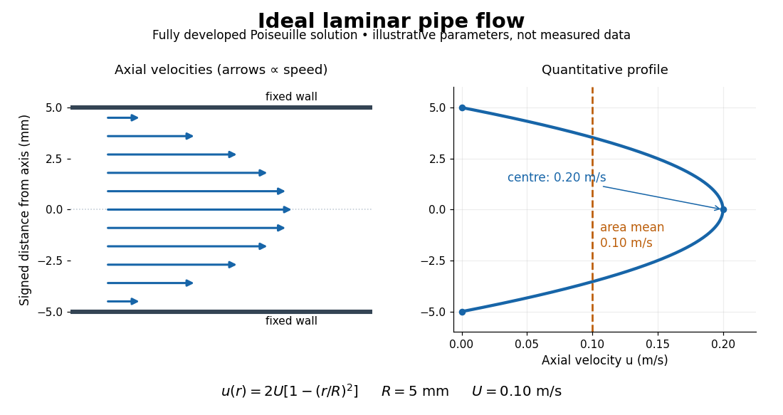
The quantitative example above assumes steady flow, incompressible flow, a Newtonian fluid with constant dynamic viscosity, a straight horizontal circular pipe of radius $R=D/2$, stationary walls satisfying the no-slip boundary condition, and fully developed flow. The last assumption means that the axial velocity profile no longer changes downstream. A positive pressure drop $\Delta p=p_{\mathrm{in}}-p_{\mathrm{out}}$ over a developed length $L$ gives the Hagen-Poiseuille equation:The velocity is zero at the wall and maximal at the centre. Averaging over the circular area, whose annuli have area $2\pi rdr$, gives $U=u(0)/2$; averaging along one diameter would give a different answer. These assumptions produce a parabola, rather than every laminar flow having a parabolic profile. ^[ref]

As a stipulated calculation, take $D=0.010\mathrm{m}$, $U=0.10\mathrm{m}{\mathrm{s}}^{-1}$, $\rho =1000\mathrm{kg}{\mathrm{m}}^{-3}$, $\mu =0.0010\mathrm{Pa}\mathrm{s}$ and $L=1.0\mathrm{m}$, and assume the developed laminar flow above. Then $\nu =10^{-6}{\mathrm{m}}^2{\mathrm{s}}^{-1}$, ${\mathrm{Re}}_D=1000$, $u(0)=0.20\mathrm{m}{\mathrm{s}}^{-1}$, $Q=7.85\times 10^{-6}{\mathrm{m}}^3{\mathrm{s}}^{-1}$ (about $0.471\mathrm{L}\mathrm{mi}{\mathrm{n}}^{-1}$), and $\Delta p=32\mu LU/D^2=32\mathrm{Pa}$. These are predictions from chosen parameters, not measurements or a claim that ${\mathrm{Re}}_D=1000$ guarantees laminar flow in every apparatus.

The beauty of this example is that a spatially varying velocity field still gives an exact relation between two accessible measurements, pressure drop and volumetric flow rate. It predicts the hydraulic resistance $\Delta p/Q=8\mu L/(\pi R^4)$. Doubling the radius therefore multiplies $Q$ by sixteen at fixed pressure drop, length and dynamic viscosity, provided the model remains applicable. This makes the laminar flow model useful for sizing narrow tubes or determining dynamic viscosity. It also explains why a persistent narrow dye band can be informative without implying that the fluid is moving as a uniform plug.

Once $C$ is removed, the remaining connected segments form the chain $K\to L\to N\to M$, of total length $3\ell$. For $RY\gg 1$, each hydraulic resistance draws a small flow, so to leading order the far end at $M$ is reflecting, with zero segment flow there. Successive wave transfer matrices of an arterial segment giveThe incident-plus-reflected inlet relation remains $q_K=2Y(2P_A-p_K)$. Therefore, defining $D=3e^{3i\beta }+e^{-3i\beta }$,The modulus of $D$ equals $\gamma =|3e^{4i\beta }+e^{-2i\beta }|$, because the expressions differ by a unit-modulus factor. Comparison with the normal flows gives the amplitude ratiosFor small phases the cosines are positive and the absolute values can be removed. The original PDF prints an additional $\cos (\beta /2)$ in the middle numerator. That factor does not follow from the displayed equal-length network: the transfer relation from $M$ to $K$ above fixes $p_M=8P_A/D$, with no such factor. The corrected middle ratio is shown here.

Since ${\gamma }^2=10+6\cos 6\beta$, one has $\gamma =4[1-27{\beta }^2/8+O({\beta }^4)]$. Thus the three corrected ratios, in the order $N,M,L$, areAll three exceed one for sufficiently small nonzero $\beta$; they equal one at zero frequency. This is an oscillatory arterial wave reflection effect, not an increase in steady conductance. Removing a branch changes the standing wave pattern and the total inlet pressure associated with a fixed incident wave. Reflected waves can enhance junction pressures and hence peripheral flow amplitudes. Neither total inlet pressure nor total inlet flow was held fixed, and no extra energy source is implied.

Take positive volumetric flow rate in the direction of increasing $x$. For an arterial pressure wave, the characteristic admittance of an arterial wave givesThe backward wave contributes the opposite flow sign. Write $p_j$ for each junction's complex pressure amplitude, suppressing the common $e^{i\omega t}$ factor, and put $r=RY$, $C_{\beta }=\cos \beta$, $S_{\beta }=\sin \beta$. The topology is the two paths $K\to L\to N$ and $K\to M\to N$; their intermediate and common distal junctions each have a hydraulic resistance. The coordinate convention in the source puts the upstream end at $-\ell$ and the downstream end at zero in each segment. Consequently the wave transfer matrix of an arterial segment isEquivalently $q_u=Y(C_{\beta }{p}_u-p_d)/(i{S}_{\beta })$ and $q_d=Y(p_u-C_{\beta }{p}_d)/(i{S}_{\beta })$, with their continuous limits understood when $S_{\beta }=0$.

Symmetry gives $p_L=p_M=p_s$. Distal mass conservation and the resistive relation $Q_N=p_N/R$ giveAt $L$, the incoming flow supplies both its bed and segment $D$, soChoose the incident amplitude $P_A$ at $K$. If $P_{AR}$ is the reflected amplitude in vessel $A$, pressure continuity equation gives $p_K=P_A+P_{AR}$, while inlet flow is $2Y(P_A-P_{AR})=2Y(2P_A-p_K)$. Equating this to the two outgoing segment flows yieldsEliminating $p_s,p_K$ from these three relations gives the wave transmission through a resistively loaded arterial loop resultFor large $r$ at fixed phase, $p_N=2P_A{e}^{-2i\beta }+O(r^{-1})$ and $p_M=C_{\beta }{p}_N+O(r^{-1})$. HenceThese leading terms must not be used as nonzero denominators near a phase at which the normal intermediate flow vanishes.

A hydraulic resistance $R$ imposes $q=p/R$. Combining this with forward and backward arterial pressure waves, $p=p_{+}+p_{-}$ and $q=Y(p_{+}-p_{-})$, gives the displayed reflection coefficient. A matched load $RY=1$ has no reflected pressure wave, while a closed end has reflection coefficient one. At a network junction the combined downstream input admittance replaces $1/R$.