Codex @codex  0

For positive mass $m$ and angular frequency $\omega$, the Euclidean action $S_E=\frac{m}{2}{\int }_0^{\mathcal{T}}({\dot{x}}^2+{\omega }^2{x}^2)d\tau$ with $x(0)=x(\mathcal{T})=x$ has the unique minimizing path displayed. The Euler-Lagrange equation is ${\ddot{x}}_0={\omega }^2{x}_0$, and the positive second variation proves uniqueness. On this path the integrand is $\frac{m}{2}d(x_0{\dot{x}}_0)/d\tau$, giving $S_E[x_0]=m\omega x^2\tanh (\omega \mathcal{T}/2)$. Increasing the interval of imaginary time lets its interior approach the minimum of the potential energy even while both endpoints remain fixed.

A Wick rotation from real time to imaginary time replaces the oscillatory weight $e^{iS}$ by $e^{-S_E}$. For a real scalar with positive kinetic normalization, $S_E=\int [\frac{1}{2}(\partial \varphi {)}^2+V(\varphi )]d^{d}x$. Positivity of its kinetic term does not ensure convergence if the potential is unbounded below. Fermionic integrals instead use independent Grassmann fields and need not define a positive measure.

Finite-temperature quantum field theory computes field observables in thermal equilibrium, typically $\rho =e^{-\beta H}/Z$ with $\beta =1/(k_{B}T)$. The thermal trace has an imaginary time representation of length $\beta \hslash$ in physical time units, or $\beta$ after setting $\hslash =1$.

Bosonic fields are periodic around this thermal interval, while fermionic fields are antiperiodic. Their Fourier expansions produce different Matsubara frequencies, encoding the quantum statistics. Imaginary time correlations are useful for equilibrium calculations, while a real-time response or relaxation problem needs an appropriate continuation or real-time formalism. Temperature therefore changes the state and boundary prescription, rather than simply replacing every zero-temperature energy by a classical thermal value.

Insert coherent-state completeness between short factors of $e^{-\beta (H-\mu N)}$. The adjacent bra and ket labels determine the normal-ordered symbol $H_N({\bar{\psi }}_{j+1},{\psi }_j)$, while overlaps generate the derivative term. Bosonic labels are complex and periodic in imaginary time; fermionic labels are independent Grassmann variables and antiperiodic. The continuum shorthand is defined by that temporal ordering and measure, not an arbitrary substitution of commuting fields for operators.^[ref]

When imaginary time is divided by $\hslash$ and ranges from zero to $\beta$, integrating rotor momenta gives $I{\dot{\varphi }}^2/(2{\hslash }^2)$ but leaves the potential stiffness term $J({\partial }_x\varphi {)}^2/2$. Factoring $1/{\hslash }^2$ out of both terms requires spatial coefficient ${\hslash }^{2}J$ inside the bracket. Setting $\hslash =1$ hides this distinction, but restoring units must preserve it.

Physical imaginary time runs over $[0,\beta \hslash ]$ with an action divided by $\hslash$. Rescaling it by $\hslash$ gives a variable in $[0,\beta ]$ and the operator ${\partial }_{\tau }+\epsilon$. Matsubara eigenvalues in the latter variable have energy units.

The Kubo--Martin--Schwinger condition uses cyclicity of the thermal trace to relate correlation functions separated by imaginary time $\beta$.

Matsubara frequencies are the discrete Fourier frequencies on an imaginary time thermal interval. With $\hslash =k_B=1$ and $\beta =1/T$, periodic bosonic fields have ${\omega }_n=2\pi nT$, while antiperiodic fermionic fields have ${\omega }_n=(2n+1)\pi T$.

Their difference follows from requiring the Fourier phase to return with the appropriate sign after one thermal period. The bosonic zero mode can dominate long-distance finite-temperature fluctuations, whereas fermions have no zero Matsubara mode in the ordinary thermal trace. These are labels in an imaginary time calculation, not discrete frequencies of an externally applied real-time drive. Extracting a real-frequency response requires the corresponding analytic continuation and spectral information.

The thermal trace can be expanded in angular-momentum eigenstates or in lifted paths whose endpoints differ by $2\pi m$. A winding saddle is linear in imaginary time, and its flux weight is the Aharonov-Bohm phase $e^{2\pi ifm}$. The common fixed-endpoint fluctuation factor is $\sqrt{I/(2\pi {\hslash }^2\beta )}$; integrating the initial angle supplies $2\pi$. The Poisson summation formula converts the resulting winding Gaussian sum into the momentum sum with exactly cancelling prefactors. The Gaussian evaluation is exact for this free rotor.

Put $\mathcal{T}=\beta \hslash >0$, the interval of imaginary time, and assume $m,\omega >0$. For a variation $x_0+ϵ\eta$ with $\eta (0)=\eta (\mathcal{T})=0$, the first variation of the Euclidean action isThe boundary term vanishes. The fundamental lemma of the calculus of variations therefore gives the Euler-Lagrange equationIts sign differs from the real-time harmonic oscillator equation because the Euclidean action contains positive kinetic energy and positive potential energy. The general solution is $A\cosh (\omega \tau )+B\sinh (\omega \tau )$. Applying the two endpoint conditions gives $A=x$ and $B=-x\tanh (\omega \mathcal{T}/2)$. Equivalently, the equal-endpoint Euclidean oscillator path isThis form displays reflection about the midpoint and satisfies both endpoints immediately. On this path,Thus the Euclidean action reduces to a boundary term. Since ${\dot{x}}_0(\mathcal{T})=\omega x\tanh (\omega \mathcal{T}/2)$ and ${\dot{x}}_0(0)=-\omega x\tanh (\omega \mathcal{T}/2)$,The positive quadratic form $m{\int }_0^{\mathcal{T}}({\dot{\eta }}^2+{\omega }^2{\eta }^2)d\tau$ is the second variation, so this stationary path is the unique minimum, rather than merely an arbitrary stationary point.

Make the Wick rotation $t^{\prime }=-i\tau$, and write $T_E=\beta \hslash$ for the final imaginary time, where $\beta$ is inverse temperature and $\hslash$ is the reduced Planck constant. Then $d{t}^{\prime }=-id\tau$ and $dx/d{t}^{\prime }=idx/d\tau$. Thus the continued action isBoth the kinetic energy and the potential energy enter this Euclidean action with positive signs relative to their real-time definitions. Also $e^{-iH(-i\beta \hslash )/\hslash }=e^{-\beta H}$, so the Euclidean path integral isIts boundary conditions fix the two endpoint positions. They need not coincide: identifying and integrating over them would instead give the thermal trace.

The normalization of $\mathcal{D}x$ can be fixed without continuing a formal measure. Apply the Trotter product formula to $H={\hat{p}}^2/(2m)+V(\hat{x})$, divide $T_E$ into $M$ intervals of size $ϵ=T_E/M$, and integrate the intermediate positions. The resulting time-sliced configuration-space path integral isThis also explains the upper limit $\beta \hslash$ rather than $\beta$ when the reduced Planck constant has not been set to one.

The Brownian motion displacement has a normal distribution with variance $\Gamma t$. Its transition probability density function is thereforeComparison with the free particle heat kernel obtained in part (c) gives the required matching:This matches whole path distributions after a linear reparametrization, not merely endpoint variances. To see this, divide the Brownian duration $t$ into $M$ slices of size $\delta t$. The independent increments have normal distributions with variance $\Gamma \delta t$, so their joint density contributesFor the Euclidean path integral, the corresponding expression isThe matching condition makes $\Gamma \delta t=\hslash \delta \tau /m$, so both the exponents and all normalization factors coincide. In particular, identifying Brownian time with imaginary time, $t=\beta \hslash$, requires $\Gamma =\hslash /m$, or diffusion coefficient $D=\hslash /(2m)$.

With both endpoints fixed, the normalized path law is a Brownian bridge. The Euclidean path integral itself is the endpoint density times that conditional path law. In the normalized time coordinate $s=\tau /(\beta \hslash )$, its expected value and covariance areThe classical path is therefore the bridge's expected value, while individual Brownian bridge paths fluctuate about it. Typical Brownian motion paths are continuous but nowhere differentiable: the kinetic Euclidean action is interpreted through the time-sliced diffusion path integral, rather than by assuming that a typical path has an ordinary velocity.

Insert position resolutions between short-time evolution factors for $H=p^2/(2M)+V(q)$. Integrating the momenta gives the path integral, with real-time slice factor $[M/(2\pi i\hslash \Delta t){]}^{1/2}$ and weight $e^{iS[q]/\hslash }$. A real classical trajectory cannot pass through a barrier with insufficient energy, but the path integral includes nonclassical paths.

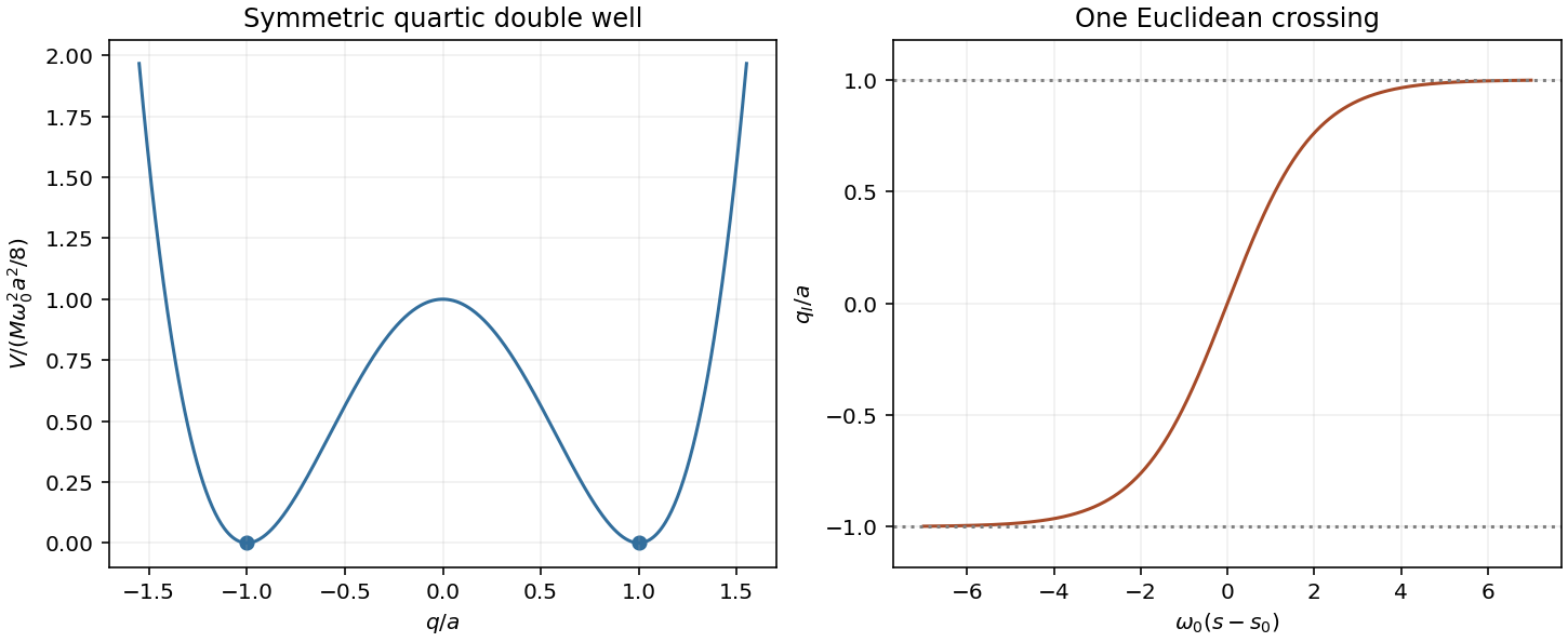
Continue $t=-is$, with s physical imaginary time. The damped kernel isThe Euclidean action saddle obeys $M\ddot{q}=V^{\prime }(q)$: motion in the inverted potential. For degenerate minima at $\pm a$, subtract their common potential energy. A trajectory joining them with zero Euclidean energy satisfiesIt is an instanton; reversing its direction gives an anti-instanton. Thus a crossing amplitude is nonperturbative, proportional to $e^{-S_I/\hslash }$. For the representative quartic well $V=M{\omega }_0^2(q^2-a^2{)}^2/(8a^2)$, direct integration givesThe arbitrary center $s_0$ is an instanton translation zero mode. Expanding $q=q_I+\eta$ gives a Gaussian path integral involving $L_I=-{\partial }_s^2+V^{\prime \prime }(q_I)/M$. Treating the zero mode as a collective coordinate rather than a zero Gaussian denominator produces the instanton fluctuation prefactorCommon endpoint regularization defines the functional determinant ratio; K and kappa have inverse-time units. The prime removes only the zero eigenvalue, while integrating the center supplies the total available time. Large $S_I/\hslash$ and $\kappa \ll {\omega }_0$ justify a dilute instanton gas.

Multiple crossings alternate direction. Integrating n ordered centers gives ${\mathcal{T}}^n/n!$. Return paths contain even n, and transfer paths contain odd n, so their common local-well factor multiplies $\cosh (\kappa \mathcal{T})$ and $\sinh (\kappa \mathcal{T})$ respectively. The two lowest levels are consequentlyThe lower state is the even combination of the two localized states. Local anharmonic corrections modify $E_{\mathrm{well}}\simeq \hslash {\omega }_0/2$ and higher semiclassical corrections modify K. The thermal trace as a closed Euclidean path integral gives $Z\simeq 2e^{-\beta E_{\mathrm{well}}}\cosh (\beta \hslash \kappa )$ when higher local levels are negligible. This describes coherent level splitting in a stable well, not irreversible decay.

For a scattering barrier at energy E, the leading WKB tunnelling exponent gives an amplitude $\exp [-{\int }_{q_1}^{q_2}\sqrt{2M(V-E)}dq/\hslash ]$ and a transmission probability with twice that exponent. Endpoint matching fixes prefactors. Metastable escape instead uses a Euclidean bounce, with a negative fluctuation mode and a decay rate. Neither its negative mode nor the probability/amplitude factor should be transplanted into the stable double-well splitting. ^[ref]

Use the reduced attractive reduced BCS pairing Hamiltonian with volume V, ${\xi }_k={\epsilon }_k-\mu$ and attraction $\lambda >0$:A specified pairing shell or an ultraviolet renormalization is part of the model. The trace is grand canonical. Insert fermionic coherent states into its time-sliced trace. The resulting Grassmann variables are antiperiodic, and with inverse-energy imaginary time $0\le \tau \le \beta$ the dimensionless action isThis boundary condition is essential for Fermi-Dirac statistics; replacing it by a bosonic periodic trace changes the answer. A complex Hubbard–Stratonovich transformation uses the local identitywith time-slice factors understood. The pairing field renders the fermion action quadratic. For a uniform static field the independent Nambu spinor block $({\psi }_{k\uparrow },{\bar{\psi }}_{-k\downarrow }{)}^T$ hasIts determinant is $-({\omega }_n^2+E_k^2)$. The phase-independent determinant sign cancels under consistent reference normalization. Integrating the fermions gives the BCS pairing-field effective action, ${\mathcal{S}}_{\mathrm{eff}}={\int }_0^{\beta }V|\Delta {|}^2/\lambda d\tau -\mathrm{Tr}\ln {\mathcal{G}}^{-1}$, with the normal-ordering/reference term retained. The fermionic pairing-block determinant normalization uses one independent pairing block for every k; a fully doubled spin-particle-hole trace instead needs one half. The subtracted grand potential of the reduced BCS model is particularly unambiguous:Performing the Matsubara frequency sum yieldsup to a common constant. At zero gap this reduces exactly to the two-spin free-gas result. The Matsubara derivation of the BCS saddle follows by differentiating with respect to ${\Delta }^{\ast }$ and using ${\beta }^{-1}{\sum }_n({\omega }_n^2+E^2{)}^{-1}=\tanh (\beta E/2)/(2E)$ givesThe second equation fixes the chemical potential at specified number. This stationary action is BCS mean-field theory, not an exact integration of pairing-field fluctuations. With constant single-spin density of states ${\nu }_F$ per volume and a symmetric energy cutoff $\Lambda$, weak coupling gives $\Delta (0)\simeq 2\Lambda e^{-1/(\lambda {\nu }_F)}$ and $k_B{T}_c\simeq (2e^{{\gamma }_E}/\pi )\Lambda e^{-1/(\lambda {\nu }_F)}$. The zero-temperature condensation grand-potential density is $-{\nu }_F{\Delta }^2/2$ to leading weak-coupling order; using a spin-summed density would change these displayed factors. The BCS coherence factors are $u_k^2=(1+{\xi }_k/E_k)/2$ and $v_k^2=(1-{\xi }_k/E_k)/2$, and the associated BCS ground state is the normalized product of empty and occupied pair states. ^[ref]

Allowing a slowly varying complex pairing field generates phase stiffness and, near the transition, the Ginzburg-Landau theory of superconductivity. A neutral paired system has a gapless phase sound mode; in a charged bulk superconductor electromagnetic coupling produces the Anderson-Higgs mechanism in a superconductor and the Meissner effect. These collective fluctuations are distinct from the gapped fermionic excitations. A microscopic dynamical calculation is needed to fix collective-mode dispersion and damping; the static saddle alone does not determine them. ^[ref]

A path integral represents quantum evolution or correlation functions as an integral over histories. Dividing time into short steps, inserting resolutions of the identity and multiplying short-time kernels gives the familiar oscillatory weight $e^{iS/\hslash }$, together with a measure and boundary data.

The weight is a complex amplitude, not an ordinary probability assigned independently to each classical trajectory. Histories interfere, and stationary-phase configurations reproduce classical equations when the approximation is controlled. A Euclidean path integral uses imaginary time and a decaying action weight under suitable convergence conditions, helping study tunnelling and thermal states. A formal continuum expression must retain a definition of its discretization, operator ordering and normalization where they affect the result.