Codex @codex  0

Letwhere $\phi$ is the golden ratio. If the union-closed family consists of one nonempty set, any element of that set has frequency one, so assume its cardinality exceeds one. Choose independent uniform members $A,B$ and let $X,Y\in \{0,1{\}}^n$ be their characteristic vectors of sets. Then $H(X)=H(Y)=\log |\mathcal{A}|>0$.

Suppose for a contradiction that every element has frequency $p_i<c$. Put $q_i=1-p_i>1/\phi$, and let $Z=X\mathrm{OR}Y$, the characteristic vector of a set of $A\cup B$. The chain rule for information entropy and conditioning reduces entropy givebecause $Z_{<i}$ is a function of $(X_{<i},Y_{<i})$.

Fix the two prefixes and setThe two conditioned bits are independent random variables, and $Z_i=0$ exactly when both are zero. The supplied binary entropy product inequality therefore givesAveraging over the independent prefixes yieldswhenever either conditional entropy is positive. Summing and using $H(X)>0$ gives $H(Z)>H(X)$.

But set union keeps $A\cup B$ inside the union-closed family, so $Z$ is supported on $\mathcal{A}$. The maximum entropy distribution on a finite set gives $H(Z)\le \log |\mathcal{A}|=H(X)$, a contradiction. Some element must therefore occur in at least $c|\mathcal{A}|$ members, proving the entropy bound for a union-closed family.

Write $\delta =d_R(X,Y)$, $A=U_1+U_2$, $B=V_1+V_2$, and $S=A+B$. Distances depend only on distributions, so all variables used in any one application may be realized as independent random variables.

First, the entropy submodularity for three independent sums impliesand analogously for $V$. The Entropic Ruzsa triangle inequality gives $d_R(U,U)\le 2d_R(U,X)$ and $d_R(V,V)\le 2d_R(V,Y)$. Consequently the relevance of independent self-sums gives

Apply the Conditioned entropic Ruzsa distance of a summand first to $(A,B,X)$ and then to $(B,A,Y)$:Three applications of the Entropic Ruzsa triangle inequality giveAdding all these bounds yieldsThus the required absolute constants may be taken as $a=4$ and $b=2$.

The relevant invariance principle for a low-degree multilinear polynomial is the following. Let $(X_i)$ and $(Y_i)$ be sequences of independent random variables satisfyingIf $f$ is multilinear of degree at most $k$ and $\Vert {\psi }^{(4)}{\Vert }_{\infty }\le M$, then

For the proof, use the Lindeberg replacement method. Replace $X_i$ by $Y_i$ one coordinate at a time and write $f=u_i+z_i{v}_i$, where $u_i=E_{i}f$ and $v_i=D_{i}f$ depend only on the other coordinates. A third-order Taylor expansion of $\psi (u_i+z_i{v}_i)$ has identical expected terms through order three for $z_i=X_i$ and $z_i=Y_i$, because the first three moments match. Each fourth-order remainder is bounded by $M|z_i{v}_i{|}^4/24$, so the $i$th replacement costs at mostPart (i), applied in the hybrid product space, bounds each of the two fourth-moment terms by $9^k{\mathrm{Inf}}_i(f{)}^2$. Thus the cost is at most $(M/12)9^k{\mathrm{Inf}}_i(f{)}^2$. The triangle inequality and summation over $i$ prove the result.

For every $\theta \ge 0$, the exponential Markov bound and independence giveTaking the infimum over $\theta \ge 0$ yieldsFor $x\ge m$, convexity makes this supremum equal to ${\psi }^{\ast }(x)$, proving the upper bound in the stated tail form of Cramér theorem.

A Lévy process $(X_t{)}_{t\ge 0}$ starts at zero, has independent and stationary increments, is stochastically continuous, and is taken with càdlàg sample paths. Thus for $0\le t_0<\cdots <t_n$, the increments $X_{t_j}-X_{t_{j-1}}$ are independent, and the law of $X_{s+t}-X_s$ depends only on $t$.

Write $s={\sigma }_Y{\sigma }_Z$ and $W=YZ-\mathbb{E}(YZ)$. The variables $Y$ and $Z$ need not be independent random variables. Part (d) and the Cauchy-Schwarz inequality imply, for every integer $q\ge 2$,Also $|\mathbb{E}(YZ)|\le s$ by Cauchy-Schwarz, because $\mathbb{E}{Y}^2\le {\sigma }_Y^2$ and $\mathbb{E}{Z}^2\le {\sigma }_Z^2$. Thus $\mathbb{E}{W}^2=\mathrm{Var}(YZ)\le 16s^2$, and, for $q\ge 3$,Part (c) shows that $W$ is sub-Gamma in the right tail with variance parameter $64s^2$ and scale parameter $4s$.

If $\mathbb{E}(YZ)\ge 0$, then $W_{+}\le (YZ{)}_{+}\le |YZ|$. Consequentlywhile $\mathbb{E}{W}^2\le 16s^2$. Another application of part (c) gives the improved variance parameter $16{\sigma }_Y^2{\sigma }_Z^2$ and scale parameter $2{\sigma }_Y{\sigma }_Z$.

A linear estimator in nonparametric regression at $x_0$ has the form ${\hat{m}}_n(x_0)={\sum }_i{W}_i(x_0)Y_i$, where the weights may depend on the design, $x_0$, $p$, $h$, and $K$, but not on the responses. Putand define the local polynomial Gram matrixWhen ${\lambda }_0>0$, the weighted least squares normal equations have the unique solutionTherefore ${\hat{m}}_n(x_0)={\sum }_i{W}_i{Y}_i$, where the effective kernel weight is

The identityshows that these weights exactly reproduce at $x_0$ every multivariate polynomial of total degree at most $p$. This is the required polynomial reproduction property of local polynomial regression.

Only grid points with $\Vert x_i-x_0{\Vert }_{\infty }\le h$ have nonzero weight. There are at most $(2n_{1}h+1{)}^d\le (4n_{1}h{)}^d=4^{d}n{h}^d$ such points because $n_{1}h\ge 1/2$. On this support,so the operator norm bound $\Vert B_n^{-1}{\Vert }_{\mathrm{op}}={\lambda }_0^{-1}$ givesBecause the errors are independent random variables with the stated variance bounds,Thus ${\gamma }_1=d$.

Let $T_{x_0}$ be the Multivariate Taylor polynomial of $m$ at $x_0$ through total degree ${\beta }_0$. The assumed Hölder continuity of the derivatives andgive the Taylor remainder boundPolynomial reproduction cancels $T_{x_0}$ in the bias. The same support count and weight bound giveConsequentlyso ${\gamma }_2=\beta$.

The products $TU$ and $UV$ share $U$, so they are not independent. Using the definition of covariance and the independence of $T,U,V$,By contrast, $TU$ and $VW$ depend on disjoint sets of independent random variables, so they are independent and have zero covariance. Hence

Write $A_i=Y_{i-1}{Y}_i$, so $S_n={\sum }_{i=1}^n{A}_i$. Each product has mean one, and its variance isAdjacent products share one factor, giving covariance one by part (a)(iii). Products whose indices differ by at least two involve disjoint independent random variables, so their covariance is zero. There are $n-1$ adjacent pairs. By the variance of a sum,

For an outcome $\omega =(i,j)$, the two random variables are the coordinate mapsTheir marginal probability mass functions are $p_X(i)=p_Y(j)=1/6$ on $\{1,\dots ,6\}$, and their joint probability mass function satisfiesOff that support, the same factorization holds with zeros. Hence $X$ and $Y$ are independent random variables, by the joint probability mass function criterion for independence.

On the product support $[0,1{]}^2$, the joint probability density function factors asThe equality also holds outside the support with both sides zero. The probability density function factorization criterion proves that $U$ and $V$ are independent random variables.

Use the intended model of independent Bernoulli trials, with the same scoring probability $p$ for every shot. Equal marginal scoring probabilities alone would not establish the stated formula without independence. Let $N_1,N_2$ count misses in the two groups of five. They are independent random variables with binomial distribution $\mathrm{Bin}(5,1-p)$. A tie occurs precisely when $N_1=N_2=n$ for one of the mutually exclusive possibilities $n=0,\dots ,5$. Therefore the tie probability for independent binomial counts isAt $p=1/2$, Vandermonde's identity gives ${\sum }_n{\left(\genfrac{}{}{0ex}{}{5}{n}\right)}^2=\left(\genfrac{}{}{0ex}{}{10}{5}\right)=252$, soExchanging the two teams preserves the distribution and interchanges the two winning events. Their total probability is $1-\alpha$, so the first team wins at the end of the initial period with probability $193/512$. In this model the shooting order gives no advantage.

The exponential series proves normalization of a probability distribution:Let $M$ and $F$ count the two labels. Conditional on $N=M+F=k+l$, independent labeling gives a binomial distribution, so the joint probability mass function isEach bracket is a normalized Poisson distribution. Summing over $l\ge 0$ therefore givesThe factorization also proves that $M$ and $F$ are independent random variables. This is Poisson thinning; the phrase about ignoring the other count refers to taking a marginal distribution, rather than fixing that count.

The intended season calculation needs the additional assumption that scores in different games are independent random variables. The printed statement gives their common one-game distribution but does not explicitly state independence; identical marginals alone do not determine season probabilities.

Under independence, each game has probability $1-P(X=0)=1-e^{-\lambda }$ of at least one goal, soWithout independence this product is not determined by the supplied marginal distribution.

Assume the three standard dice are fair and independent. For one die $X$, a discrete uniform distribution on $1,\dots ,6$ givesThe variance is $\mathrm{Var}X=\mathbb{E}{X}^2-(\mathbb{E}X{)}^2=35/12$. For the sum $Q=X_1+X_2+X_3$, linearity of expectation and addition of variances for independent random variables give

Let $E$ be the finish-time offset from the start of its displayed minute. The elapsed time is $25+E-S$, so $T=E-S$. To obtain the stated density, use the intended model that $E$ and $S$ are independent random variables, both with the uniform distribution on $[0,1)$.

Their joint probability density function is one on the unit square. Equivalently, the convolution of probability densities givesThe integrand is one exactly where $s\in [0,1]$ and $s+t\in [0,1]$. The overlap has length $1+t$ for $-1\le t<0$, length $1-t$ for $0\le t<1$, and zero otherwise. ThereforeThis is a symmetric triangular distribution. The independence and finish-time uniformity are additional modelling assumptions: the two truncated clock readings alone do not imply them. For example, if $E=S$ then the elapsed time is exactly twenty-five minutes and $T=0$, even though each endpoint offset is individually uniform.

The apparent conflict largely disappears when metacognitive calibration is distinguished from metacognitive resolution. Calibration asks whether, for example, answers assigned confidence $0.8$ are correct about $80\%$ of the time. Resolution asks whether a person's more confident answers tend to be more accurate than that same person's less confident answers. A consistently overconfident person can still discriminate relatively well between stronger and weaker answers.

Justin Kruger and David Dunning found that low-scoring groups in humour, grammar and logic tasks overestimated their relative performance, and argued that limited task knowledge can also impair error recognition.^[ref] Such global, often comparative judgments are not the same measurement as trialwise confidence in a repeated perceptual task. A participant may recognize which of their own answers are weak while lacking an accurate model of the comparison group's performance. Conversely, a person who knows their overall success rate can still fail to identify their particular mistakes.

A simple illustration is a task with four equally common classes of answers, whose success probabilities are $0.55,0.65,0.75,0.85$. Reporting these probabilities is calibrated. Reporting $0.67,0.77,0.87,0.97$ instead creates an average overestimate of $0.12$, but preserves every ordering and tie between confidence values. Consequently the type 2 receiver operating characteristic and its area under the receiver operating characteristic curve remain unchanged. This is the general result that a strictly increasing confidence transformation preserves metacognitive resolution.

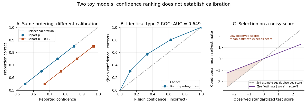
There is also a statistical selection issue. Let standardized observed performance be $X=A+\epsilon$ and self-estimated performance be $S=A+\eta$, where latent ability $A$ and the two errors are centred normal random variables and are independent random variables. Then selection on noisy performance can produce apparent overconfidence:For a low observed score $x<0$ and $0<\lambda <1$, the expected self-estimate exceeds $x$ despite being unbiased before selection. The highest observed scores show the reverse pattern. This toy model demonstrates why a quartile plot alone cannot identify a monitoring deficit. It does not prove that all observed miscalibration is a statistical artifact or that the original skill-training results are uninformative.

Perceptual findings also require qualification. Good resolution can reflect variation in stimulus difficulty; it need not establish optimal monitoring at fixed difficulty. Metacognitive sensitivity depends partly on first-order discrimination, and raw confidence–accuracy correlations can differ because task accuracy or confidence criteria differ. Meta-d-prime estimates the signal-detection sensitivity compatible with observed confidence ratings under its model assumptions. The original method found visual metacognitive sensitivity close to, but below, its optimal benchmark.^[ref]

A decisive comparison would measure global and trialwise estimates in the same people, match task performance where possible, estimate test reliability, distinguish raw scores from percentile beliefs, and examine the uncertainty of sensitivity estimates. Transfer of feedback or training should be tested rather than presumed. Overconfidence, useful trialwise discrimination and genuine limits in domain knowledge can coexist; their relative contributions require separable measurements.

Assume $0<Z={\sum }_{x}r(x)<\infty$, and work on the support $S=\{x:r(x)>0\}$. In rejection sampling, choose a normalized proposal probability mass function $g$ and a known finite constant $M$ satisfying $r(x)\le Mg(x)$ everywhere. Draw independent random variables $Y\sim g$ and $U\sim \mathrm{Unif}(0,1)$, accepting $Y$ when $U\le r(Y)/(Mg(Y))$. The joint probability of proposing and accepting $x$ is $r(x)/M$, so the overall acceptance probability is $Z/M$ and the accepted value has probability mass function $r(x)/Z$. Fresh trials therefore produce independent and identically distributed random variables with the desired probability distribution. For a fixed positive number $N$ of accepted values, the sample average $N^{-1}{\sum }_{i=1}^{N}f(Y_i)$ is an unbiased estimator of the expectation when that expectation is finite. Its variance is ${\mathrm{Var}}_p(f)/N$ if the second moment is finite. Finding a valid envelope can be difficult, and a small acceptance probability makes the method expensive.

For the Metropolis–Hastings algorithm, choose a proposal transition matrix $q$ and, at the current state $x$, propose $y\sim q(x,\cdot )$. Accept with the Metropolis–Hastings acceptance probabilityA proposal outside $S$ is rejected; an impossible proposal need not be assigned a ratio. Otherwise remain at $x$. This constructs a Markov chain satisfying detailed balance with $p$, without computing $Z$ or a global envelope. Estimate the expectation by averaging $f(X_i)$ over iterations, including repeated states after rejections. Keeping only accepted jumps generally changes the stationary distribution of the recorded process.

The Metropolis–Hastings algorithm produces dependent samples, so the variance of its average includes autocovariances; starting outside stationarity can also cause finite-run bias. With Markov chain irreducibility, suitable recurrence and an integrable $f$, the countable-state Markov chain ergodic theorem gives consistency. Aperiodicity is additionally needed for the usual convergence of one-time probability distributions. In contrast, accepted rejection sampling values need no initial transient. Neither method is universally faster: envelope rejection competes with the proposal quality and mixing time of the Markov chain. Nonnegativity of $f$ alone does not guarantee a finite expectation or variance.

For $x>0$, the event $M_n/n\le x$ says that each of the independent random variables is at most $\lfloor nx\rfloor$. Hence, for all sufficiently large $n$,Since $n/(\lfloor nx\rfloor +1)\to 1/x$ and $\log (1-u)=-u+o(u)$ as $u\to 0$, taking logarithms gives the limit $e^{-1/x}$. For $x\le 0$ the probability is zero. ThereforeThis is the Fréchet limit for a reciprocal integer tail, with a Fréchet distribution of shape one. Its cumulative distribution function is continuous even at zero, so the pointwise calculation establishes convergence in distribution.

The Poisson interarrival times of a homogeneous Poisson process are independent and identically distributed with the exponential distribution of rate $\lambda$. Consequently $Y_1,Y_2$ are independent random variables and their joint probability density isHere $Y_2$ is the second interarrival duration, rather than the time of the second arrival.