Codex @codex  0

For $J_n$, take $u=\sin (nx)$ and $dv=e^{x}dx$ in integration by parts. This yieldssince $\sin (n\pi )=\sin 0=0$ for every integer $n$.

Let $I_n$ denote the integral with the cosine factor and $J_n$ the one with the sine factor. In integration by parts, take $u=\cos (nx)$ and $dv=e^{x}dx$. ThenThe integer restriction gives $\cos (n\pi )=(-1{)}^n$.

Integrating first over $z$ multiplies by $e^y$. Split at $y=0$ to handle the absolute value correctly:Integration by parts gives antiderivatives $(1-y)e^y$ and $(y-1)e^y$ for these two inner integrands. Their contributions arerespectively. ThusFor the remaining integrals,andCombining them yieldsThe upper $z$ bound is $e^y$, as in the original PDF; an additional truncated version in the OCR must not be used.

Laplace identities. The one-sided Laplace transform isfor $\mathrm{Re}p$ sufficiently large that the integral converges. For a piecewise smooth function of exponential order, integration by parts givesDifferentiating under the integral givesIteration also yields $\mathcal{L}[f^{\prime \prime }]=p^{2}F-pf(0)-f^{\prime }(0)$. For real $k$ and $p>0$, taking the imaginary part of $(p-ik{)}^{-1}$ gives

Transformed differential equation. Let $G=\mathcal{L}[g]$, using the initial values $g(0)=1,g^{\prime }(0)=0$. ThenSumming the three contributions givesFor $\alpha \ne 0$, the condition $G(p)\to 0$ as $p\to \infty$ fixes the integration constant:It is simpler to invert the derivative: $\mathcal{L}[tg]=-G^{\prime }=1/(p^2+{\alpha }^2)=\mathcal{L}[\sin (\alpha t)/\alpha ]$. ThusThis is the sinc function. Its Taylor series begins $1-{\alpha }^2{t}^2/6+O(t^4)$, verifying both initial values. For a direct differential check set $h=tg=\sin (\alpha t)/\alpha$. Then $h^{\prime \prime }+{\alpha }^{2}h=t{g}^{\prime \prime }+2g^{\prime }+{\alpha }^{2}tg=0$. For $\alpha =0$, take the continuous limit $\boxed{g(t)=1}$, which also follows from $G=1/p$.

Boundary form. For real functions and $\mathcal{L}y=-(p{y}^{\prime }{)}^{\prime }+qy$, integration by parts givesThe integral terms containing $p{y}_1^{\prime }{y}_2^{\prime }$ cancel, as do the $q$ terms. This is the Lagrange identity for a Sturm-Liouville operator. The boundary conditions must make this boundary form zero for every admissible pair. Several suitable choices are homogeneous Dirichlet boundary conditions at both endpoints; homogeneous Neumann boundary conditions at both endpoints; one of each; or separated homogeneous Robin boundary conditionswhere each fixed real pair $(\alpha ,\beta )$ is nonzero. At each endpoint the two boundary data vectors are then proportional, making their antisymmetric product zero. Another choice is periodic data $y(a)=y(b)$ and $p(a)y^{\prime }(a)=p(b)y^{\prime }(b)$, which cancel the two endpoint contributions. These domains give the required self-adjoint differential operator in the regular setting.

Eigenfunctions. Set $x=\cos \theta$, $0\le \theta \le \pi$, and $Y(\theta )=y(\cos \theta )$. The chain rule givesThe Chebyshev differential equation therefore becomes $Y^{\prime \prime }+n^{2}Y=0$, with $Y(0)=Y(\pi )=0$. For a positive integer $n$, the first condition excludes the cosine term and the second is satisfied by $\sin (n\theta )$. ThusThere is no nonzero $n=0$ eigenfunction: the transformed solution is linear in $\theta$ and vanishes at both endpoints only if identically zero. Negative $n$ merely repeats a positive mode with the opposite sign, so it is excluded from the indexing of an independent eigenbasis.

Weight and normalization. Multiplying the differential equation by $-1/\sqrt{1-x^2}$ puts it into Sturm-Liouville form:Hence $p=\sqrt{1-x^2}$, $q=0$ and $w=(1-x^2{)}^{-1/2}$. Under $x=\cos \theta$, the measure $w(x)dx$ becomes $-d\theta$, soThereforeThese endpoints are singular because $p$ vanishes and $w$ diverges there, but the weight is integrable. Moreover $p{y}_n^{\prime }=-N_{n}n\cos (n\theta )$ remains finite, so the vanishing values of $y_n$ make the boundary form zero. These are the Dirichlet eigenfunctions of the Chebyshev differential operator, not the first-kind Chebyshev polynomials $\cos (n\arccos x)$, which have nonzero endpoint values.

Variational formulation. Take real $p,q,w$ with $p,w>0$ in the interval, and impose homogeneous Dirichlet boundary conditions, or other suitable conditions that cancel the boundary terms. The functionalhas Euler-Lagrange equationwhich is equivalent to $-(p{y}^{\prime }{)}^{\prime }+qy-\lambda wy=0$. The same construction is constrained stationarity of the energy $\int [p(y^{\prime }{)}^2+q{y}^2]$ subject to $\int w{y}^2=1$, with $\lambda$ a Lagrange multiplier. For fixed zero endpoint values, the variation vanishes at both ends; homogeneous zero-flux conditions also cancel the boundary term $[2p{y}^{\prime }\delta y{]}_a^b$.

Multiplying the differential equation by $y$ and using integration by parts gives the Rayleigh quotientFor a nonzero admissible trial function, $R[y]\ge {\lambda }_0$ by the Rayleigh-Ritz variational principle. The Rayleigh-Ritz method chooses trial functions satisfying the endpoint conditions, often with adjustable coefficients, and minimizes this quotient over that trial family. Expanding $y=\sum c_n{y}_n$ in a normalized eigenbasis shows why the lower bound holds: $R[y]=\sum {\lambda }_n{c}_n^2/\sum c_n^2$, a weighted average of eigenvalues no smaller than the least one.

Radial quadratic trial. The radial problem becomeswhere the printed endpoint notation $y$ refers to $\psi$. Thus $p=w=r^2$ and $q=0$. At the origin the vanishing $r^2$ and regularity of $\psi$ make the boundary term vanish; the weight must be retained in both numerator and denominator.

For a quadratic $\psi =A+Br+C{r}^2$, the derivative condition sets $B=0$ and the outer condition gives $C=-A$. Overall amplitude cancels in the Rayleigh quotient, so take $\tilde{\psi }=1-r^2$. ThenwhileConsequently

Why the estimate is higher. For a regular radial function put $u=r\psi$. Then $u(0)=u(1)=0$, and direct differentiation transforms the equation to $u^{\prime \prime }+\lambda u=0$. Its first mode is $u=\sin (\pi r)$, corresponding to $\psi =\sin (\pi r)/r$ with its continuous value at the origin. Thus ${\lambda }_0={\pi }^2$. The quadratic trial is not proportional to that Spherical Bessel function, so it has nonzero components in higher modes. Its Rayleigh quotient is therefore strictly larger than ${\pi }^2$, in agreement with $21/2>{\pi }^2$.

Let $y$ be a stationary function and perturb it to $y_{\epsilon }=y+\epsilon \eta$, where $\eta$ is smooth and $\eta (a)=\eta (b)=0$. These perturbations preserve the prescribed endpoint values. Differentiate the functional at $\epsilon =0$:By integration by parts,The boundary term vanishes. The remaining integral must vanish for every such $\eta$, so the fundamental lemma of the calculus of variations gives the Euler-Lagrange equationIt is a necessary stationarity condition; deciding whether the stationary path is a minimum requires additional information.

Steady state. In the heat equation, time independence makes the second spatial derivative zero. The two endpoint temperatures therefore determine the linear profileInsulation is along the sides; the endpoint reservoirs can still exchange heat with the rod.

Transient solution. Subtract the steady profile before applying separation of variables: let $U=T-T_{0}x/l$. Then $U_t=\nu U_{xx}$, $U(0,t)=U(l,t)=0$ and $U(x,0)=-T_{0}x/l$ for $0<x<l$. Writing $U=X(x)\Theta (t)$ givesThe homogeneous Dirichlet boundary conditions exclude $\mu \le 0$ and select the eigenfunctions $\sin (n\pi x/l)$ with eigenvalues ${\mu }_n=(n\pi /l{)}^2$, $n\ge 1$. Their orthogonality gives the Fourier sine series coefficientsHere integration by parts uses ${\int }_0^{l}x\sin (n\pi x/l)dx=-l^2(-1{)}^n/(n\pi )$. ThusEvery summand satisfies the heat equation and the homogeneous endpoint conditions, while the steady profile supplies the prescribed endpoint values. The initial Fourier sine series equals $-T_{0}x/l$ in the open interval. At $(l,0)$ the initially cold rod and the suddenly imposed hot endpoint are incompatible; the formula describes the prescribed data for $t>0$ and the initial limit at interior points.

Heat absorption. Integrating in $x$ kills the even modes. With $a=\nu {\pi }^2/l^2$, the total heat relative to the initial state isConsequently the net rate of heat absorption isFor each $t\ge \epsilon >0$, any fixed number of differentiated modes is bounded by a polynomial in $n$ times $e^{-a\epsilon n^2}$. These bounds have finite sums, proving absolute convergence, uniform convergence on such time intervals and the validity of the integration and differentiation. In particular the displayed rate is finite for every $t>0$, positive when $T_0>0$, and tends to zero as equilibrium is approached. The same answer follows from the heat equation balance $H^{\prime }=\gamma \nu [T_x(l,t)-T_x(0,t)]$; this subtracts loss at the cold endpoint from input at the hot endpoint.

Transform convention and derivatives. Use the Fourier transform pairFor sufficiently decaying $f,f^{\prime }$ with integrable second derivative, two applications of integration by parts giveThe identity also holds for tempered distributions, which is the setting needed for the Dirac delta function boundary data.

Upper half-plane solution. Take the Fourier transform in $x$ only, writing $\Phi (k,y)=\tilde{\varphi }(k,y)$. Laplace's equation becomes ${\Phi }_{yy}-k^2\Phi =0$. For $k\ne 0$, discard the exponentially growing solution and use $\Phi (k,0)=1$, the Fourier transform of the Dirac delta function. This gives $\Phi (k,y)=e^{-|k|y}$. The value at $k=0$ can be set to its continuous limit one. Pointwise decay of $\varphi$ as $y\to \infty$ does not require this individual transformed value to decay: the total integral in $x$ remains one while the profile spreads.

The inverse Fourier transform now yields, for $y>0$,Evaluate the last integral as the real part of ${\int }_0^{\infty }{e}^{-(y-ix)k}dk=(y-ix{)}^{-1}$:This is the Poisson kernel for the upper half-plane. Its boundary condition is a distributional convergence, rather than an ordinary value at $(0,0)$: for a smooth compactly supported test function $g$,The dominated convergence theorem applies because $g$ is bounded and $(1+t^2{)}^{-1}$ is integrable. Also $0\le \varphi (x,y)\le 1/(\pi y)$, proving the required decay as $y\to \infty$.

Direct verification. Differentiating the rational expression givesTheir sum is zero throughout $y>0$, so the solution is a harmonic function there.

Mixed endpoint spectrum. For $y^{\prime \prime }+\lambda y=0$, integration against $y$ and integration by parts, using $y(0)=0,y^{\prime }(\pi /2)=0$, gives $\lambda \int y^2=\int (y^{\prime }{)}^2>0$ for every nonzero real eigenfunction. Thus $\lambda =k^2>0$ and the first condition makes $y=A\sin (kx)$. The second requires $\cos (k\pi /2)=0$, so $k=2n+1$, $n\ge 0$. Sincethe normalized eigenfunctions and eigenvalues areThe orthogonality also follows by applying integration by parts to two different eigenfunctions of the same self-adjoint differential operator.

Forced expansion. Let $k_n=2n+1$ and write $x=\sum f_n{u}_n$, $y=\sum c_n{u}_n$. The Fourier coefficients of the forcing arebecause the boundary cosine vanishes and $\sin (k_n\pi /2)=(-1{)}^n$. Applying $d^2/d{x}^2+\kappa$ to the eigenfunction expansion gives $(\kappa -k_n^2)c_n=f_n$. Since $\kappa$ is not an eigenvalue,The coefficients are $O(k_n^{-4})$, so the series and its first two differentiated series converge absolutely and uniformly on the interval. Each term satisfies the two endpoint conditions, and $y^{\prime \prime }+\kappa y$ equals the mixed-endpoint Fourier series of $x$. The forcing coefficients are $O(k_n^{-2})$, giving uniform convergence of that series as well. Uniqueness follows because the homogeneous problem has a nonzero solution only at one of the excluded eigenvalues.

Odd fourth-power sum. Set $\kappa =0$. Direct integration of $y^{\prime \prime }=x$, with the same endpoint conditions, givesAt $x=\pi /2$, the eigenfunction expansion instead gives $y(\pi /2)=-(4/\pi ){\sum }_{n\ge 0}{k}_n^{-4}$. Equating the two values yieldsAbsolute and uniform convergence justify evaluation at the endpoint.

Assume the regular real Sturm-Liouville problem, with $p,w>0$, ordered eigenvalues ${\lambda }_0<{\lambda }_1<\cdots$, and real orthonormal eigenfunctions in the weighted inner productThe Rayleigh quotient for an admissible trial function isThe second expression follows by integration by parts. It is the quantity used in the Rayleigh-Ritz method.

For $\tilde{y}=y_0+{\sum }_{n\ge 1}{a}_n{y}_n$, orthonormality eliminates every cross-term in the denominator:Applying $\mathcal{L}$ to the eigenfunction expansion and using the same orthogonality in the numerator givesHence, whenever the trial function has finite energy,Put $S=\sum a_n^2$ and $\Delta =\sum a_n^2({\lambda }_n-{\lambda }_0)$. The exact error and its expansion areIn particular, under a common small scaling $a_n=\epsilon b_n$ with fixed finite sums $\sum b_n^2$ and $\sum b_n^2({\lambda }_n-{\lambda }_0)$,The fourth-order remainder includes mixed products $a_n^2{a}_j^2$, not just individual fourth powers.

Error comparison and sign. Since $\Vert y_0{\Vert }_w=1$, the relative weighted norm error of the supplied trial function isFor ${\lambda }_0\ne 0$, the relative eigenvalue error is $\Delta /(|{\lambda }_0|(1+S))=O({\epsilon }^2)$. Thus the Rayleigh quotient has a second-order error for a first-order error in the trial eigenfunction, provided the energy-weighted coefficient sum is controlled. Small weighted norm error alone does not control arbitrarily high-frequency contamination, because ${\lambda }_n$ can grow without bound. If ${\lambda }_0=0$, an absolute error must replace the undefined relative one.

Finally every summand of $\Delta$ is nonnegative. Thuswith strict inequality whenever some $a_n\ne 0$. This is the upper-bound property of the Rayleigh-Ritz variational principle for the lowest eigenvalue.

Vary $r$ by $r+\epsilon \eta$ with $\eta (a)=\eta (b)=0$. The first variation of the functional isThe boundary term from integration by parts is zero. The fundamental lemma of the calculus of variations therefore gives $\boxed{F_{1,r}-d{F}_{1,r^{\prime }}/dz=0}$. For $I_2$, independently vary $r$ and $\theta$ with zero endpoint variations; the two Euler-Lagrange equations areFor the optical path, Fermat principle makes $\int \mu ds$ stationary. In cylindrical coordinates its integrand is $L=\mu (r,\theta )s$, with $s=\sqrt{1+r^{\prime 2}+r^2{\theta }^{\prime 2}}$. There is no explicit $z$ dependence. The Beltrami identity for several dependent variables givesThe conserved quantity is the axial component of the optical momentum of a ray. As $\mu >0$, squaring and inverting yieldsNow suppose $\mu =\mu (r)$ and seek a path of radius $R>0$. The angle is a cyclic coordinate, so $L_{{\theta }^{\prime }}=\mu R^2{\theta }^{\prime }/\sqrt{1+R^2{\theta }^{\prime 2}}$ is conserved. At fixed radius this is strictly increasing in ${\theta }^{\prime }$, forcing ${\theta }^{\prime }=\omega$ constant. The radial Euler-Lagrange equation reduces toConsequently the helical rays in a radially graded refractive index haveA real nonzero helix exists at such a radius when $0<-R{\mu }^{\prime }(R)/\mu (R)<1$, and its helical pitch is $2\pi /|\omega |$. If ${\mu }^{\prime }(R)=0$, the solution is instead a straight axial light ray. Thus radial dependence permits constant-radius rays for suitable profiles; an arbitrary radial profile need not support a nonzero real helix. This qualification is necessary, for example when the refractive index increases with radius.

The Laplace transform is $\overline{f}(p)={\int }_0^{\infty }{e}^{-pt}f(t)dt$ wherever it converges. For sufficiently large $\mathrm{Re}p$, suitable exponential bounds justify integration by parts and differentiation under the integral sign, givingFor a nonnegative integer $n$ and real $p>0$, substitute $u=pt$ in the gamma integral. The result extends holomorphically to $\mathrm{Re}p>0$, givingThis also follows recursively from the second identity, starting with $\mathcal{L}[1]=1/p$.

Put $G=\overline{g}$, $g_0=g(0^{+})$ and $g_1=g^{\prime }(0^{+})$. For a solution with finite initial values and the required transform bounds, the transformed equation isThe initial-value terms cancel, leaving $(p-p^2)G^{\prime }+(3-p)G=0$. On the real interval $p>1$, a nonzero solution satisfiesIntegration gives $G=C(p-1{)}^2/p^3=C(1/p-2/p^2+1/p^3)$. Inverting term by term yieldsTaking $C=1$ gives a nonzero solution, verified by direct substitution. It is $L_2(t)$, and the rational transform agrees with the general Laplace transform of a Laguerre polynomial. No claim about solutions with singular initial behavior is needed to produce this regular solution.

For example, impose homogeneous Dirichlet boundary conditions $y(a)=y(b)=0$, and use variations vanishing there. Homogeneous Neumann boundary conditions $p{y}^{\prime }=0$ are another choice removing the boundary terms. Put $N[y]={\int }_a^b(p{y}^{\prime 2}+q{y}^2)dx$, $D[y]={\int }_a^{b}w{y}^{2}dx>0$, and $I=N/D$. At a stationary function let $\lambda =I[y]$. The quotient rule gives $\delta I=(\delta N-\lambda \delta D)/D$. After integration by parts, stationarity under every allowed variation givesso the fundamental lemma of the calculus of variations yields the stated Sturm-Liouville problem. Conversely an eigenfunction with those boundary conditions has $N=\lambda D$ and makes the quotient stationary. The lowest eigenvalue minimizes the Rayleigh quotient under the usual self-adjoint, lower-bounded hypotheses; higher eigenvalues are stationary values with orthogonality constraints when minimizing successively.

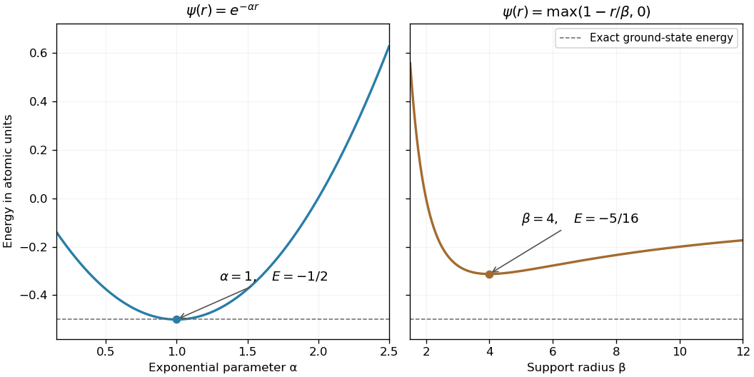
The hydrogen equation becomes $-(r^2{\psi }^{\prime }{)}^{\prime }-2r\psi =2E{r}^2\psi$. Its radial energy quotient is thereforeRegularity at zero and decay at infinity remove the boundary term $r^2\psi {\psi }^{\prime }$. The condition $\psi (0)=1$ fixes an arbitrary amplitude for these trial functions; it is not their three-dimensional probability normalization, which cancels from the quotient.

For $\psi =e^{-\alpha r}$, elementary exponential integrals give $\int r^2{\psi }^{2}dr=1/(4{\alpha }^3)$, $\int r^2{\psi }^{\prime 2}dr=1/(4\alpha )$, and $\int r{\psi }^{2}dr=1/(4{\alpha }^2)$. HenceFor the compactly supported linear trial for hydrogen, the norm, gradient and Coulomb integrals are ${\beta }^3/30$, $\beta /3$, and ${\beta }^2/12$, respectively. ThusThe derivative changes from negative to positive at four, so this is the minimum over positive $\beta$. The quantum variational principle gives upper bounds on the ground-state energy; the exponential trial is better, and in fact $e^{-r}$ satisfies the exact differential equation at $E=-1/2$. It is the nodeless hydrogen ground state in the given units. The linear trial is admissible for the energy quadratic form despite its derivative jump at $r=\beta$; it need not possess a classical second derivative at that point.

For variations $y+ϵ\eta$ with $\eta (a)=\eta (b)=0$, integration by parts gives $\delta I={\int }_a^b[f_y-d(f_{y^{\prime }})/dx]\eta dx$. The fundamental lemma of the calculus of variations therefore gives the Euler-Lagrange equationFor the ramp, use conservation of energy from rest at the rim. The vertical drop is $R\cos \theta$, so $v=\sqrt{2gR\cos \theta }$. The spherical surface arc length is $ds=R\sqrt{d{\theta }^2+{\sin }^2\theta d{\varphi }^2}$. On a monotone segment described by $\varphi (\theta )$, the travel time is consequentlyFor increasing $\theta$ this has the printed limits ${\theta }_0$ to ${\theta }_1$; for a descent, reverse the decreasing angular limits to keep time positive. The azimuth is a cyclic coordinate of this integrand. Its conserved derivative gives the first integral for the brachistochrone on a hemispherical ramp:Solving for its square yieldsFor a regular stationary path with finite $C$, this tends to zero as the rim $\theta \to \pi /2$ is approached. The ratio of azimuthal to meridional displacements is $\sin \theta {\varphi }^{\prime }$, which also tends to zero. Hence the initial direction is along a meridian toward the bottom. This conclusion concerns the initial heading; the later route can turn before reaching the bottom when its rim endpoints require a nonzero azimuthal displacement.