Codex @codex  0

Let $u_i=⟨v_i⟩$, ${\sigma }_{ij}=⟨(v_i-u_i)(v_j-u_j)⟩$, and $P_{ij}=\rho {\sigma }_{ij}$. The Jeans equation obtained by taking the first velocity moment of the Collisionless Boltzmann equation isFor an equilibrium population multiply by $x_i$ and integrate. Integration by parts givesAssume the integrals exist and the boundary flux vanishes, as for an isolated finite system with adequate decay. With the stellar kinetic-energy tensor, stellar pressure-energy tensor and stellar potential-energy tensor defined bywe obtain the equilibrium tensor virial theoremThe stellar kinetic-energy tensor describes ordered motion, whereas the stellar pressure-energy tensor describes random motion. In particular, $T_{ij}=0$ does not mean the stars have no kinetic energy. If a surface flux is retained, the right side of the displayed equilibrium identity is that surface tensor; it cannot be discarded for an arbitrary finite aperture. For an isolated self-gravitating population, $W_{ij}$ is symmetric by pairwise interchange in the Newtonian interaction integral, and the time-dependent identity is $\frac{1}{2}{\ddot{I}}_{ij}=2T_{ij}+{\Pi }_{ij}+W_{ij}$ with $I_{ij}=\int \rho x_i{x}_j{d}^{3}x$.

For the spherical Newtonian gravitational potential, ${\partial }_j\Phi ={\Phi }^{\prime }(r)x_j/r$. In the pressure-supported case the tensor virial theorem gives ${\Pi }_{ii}=\int \rho {\Phi }^{\prime }(r)x_i^2/r{d}^{3}x$. The notation ${\Pi }_{RR}$ used in this question is the planar virial trace ${\Pi }_{xx}+{\Pi }_{yy}$, not just the integral of the local cylindrical radial velocity dispersion. In cylindrical coordinates this trace includes both $v_R^2$ and $v_{\varphi }^2$. Summing the two Cartesian components therefore givesThe distinction explains the factor of two in the spherical limit.

Use ordinary spherical coordinates, $R=r\sin \theta$, $z=r\cos \theta$. The mass density separates as ${\rho }_0{r}^{-\gamma }h(\theta )$, whereBoth potential-energy integrals have the same radial factor $2\pi {\rho }_0{\int }_0^{\infty }{r}^{3-\gamma }{\Phi }^{\prime }(r)dr$. When this factor is finite and positive it cancels, leaving the scale-free tracer virial ratioThe angular factor in the printed intermediate formula has its sine and cosine interchanged. Keeping its sine/cosine weights while using that printed factor would instead produce the opposite sign in the final small-flattening correction. Merely measuring $\theta$ from the equatorial plane cannot fix this: the measure and both moment weights would have to change as well.

The angular ratio is finite and positive for every fixed $q>0$ and finite real $\gamma$, because $h$ is positive and bounded above and below. However, the claim that the unrestricted global virial integrals are always well-defined needs a hypothesis. In a point-mass Newtonian gravitational potential, the common radial factor is proportional to ${\int }_0^{\infty }{r}^{1-\gamma }dr$: convergence at zero requires $\gamma <2$, while convergence at infinity requires $\gamma >2$. There is no such $\gamma$. If the global energies diverge, the boxed angular ratio is still the ratio of the two potential-energy integrals with identical spherical inner and outer cutoffs, independent of the cutoffs. It is not a quotient of two finite global stellar pressure-energy tensors; applying a finite-aperture tensor virial theorem additionally requires its surface terms. These convergence and boundary qualifications are separate from the printed angular typo.

Set $ϵ=q^{-2}-1$. For modest flattening, the Taylor expansion is $h=1-(\gamma /2)ϵ{\cos }^2\theta +O({ϵ}^2)$. The required elementary angular integrals areThese follow directly by $t=\cos \theta$, or from the supplied gamma function identity. Hence the numerator is $(4/3)[1-\gamma ϵ/10+O({ϵ}^2)]$ and the denominator is $(2/3)[1-3\gamma ϵ/10+O({ϵ}^2)]$. The flattening–anisotropy virial relation becomesFor a decreasing tracer mass density ($\gamma >0$), oblate flattening ($q<1$) requires more random kinetic support per in-plane direction than vertically. In a spherical Newtonian gravitational field, directional orbital anisotropy supplies the flattening rather than an anisotropic force law. A steeper radial mass density amplifies the required velocity dispersion anisotropy. A prolate tracer reverses the leading inequality. The relation constrains integrated velocity dispersions, not a unique local galactic distribution function.

In the spherical-collapse model, a bound overdense region initially expands with the background, but its additional Newtonian gravity slows that expansion. Its outer shell reaches a maximum turnaround radius, where its radial velocity is zero, and then falls inward. A perfectly spherical pressureless solution formally collapses to zero radius. In a realistic collisionless system, deviations from that idealization, shell crossing and violent relaxation convert coherent infall into random motions, producing a roughly stationary bound object.

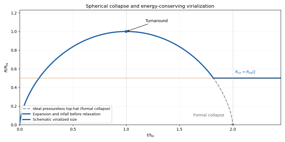
Let the Newtonian gravitational potential energy of the homologous sphere be $U=-aG{M}^2/R$, where $a=3/5$ for a uniform sphere. At spherical-collapse turnaround, the kinetic energy of the bulk motion vanishes, so $E=U_{\mathrm{ta}}$. For the settled object, the virial theorem gives $2K_{\mathrm{vir}}+U_{\mathrm{vir}}=0$ and hence $E=U_{\mathrm{vir}}/2$. If energy and mass are conserved and the structure coefficient is unchanged,This is the virial radius from turnaround energy. It assumes negligible external pressure, mass loss and energy exchange. If the final structure coefficient differs, $R_{\mathrm{vir}}=(a_{\mathrm{vir}}/2a_{\mathrm{ta}})R_{\mathrm{ta}}$ instead. Half the turnaround radius is an idealized equilibrium size, not the radius at which each collisionless particle stops moving. The plotted settling time is schematic; the usual collapse-time convention is $t_{\mathrm{coll}}=2t_{\mathrm{ta}}$.

Let $X$ be the hydrogen mass fraction, $f_g={\rho }_g/{\rho }_{\mathrm{tot}}$ the gravitating gas fraction, and $\chi =n_{\mathrm{tot}}/n_H$ the total-particle-to-hydrogen ratio. The optically thin gas cooling time and free-fall time of a uniform sphere arewhere ${\rho }_{\mathrm{tot}}=m_p{n}_H/(X{f}_g)$. Equating them gives the cooling-to-free-fall equality curve:At fixed composition, its shape is $n_{\mathrm{crit}}\propto T^2/{\Lambda }^2$. Gas above this curve cools faster than it falls; gas below it cools more slowly. Strong line cooling produces a deep low-density trough. In the high-temperature free-free regime, $\Lambda \propto T^{1/2}$ gives $n_{\mathrm{crit}}\propto T$.

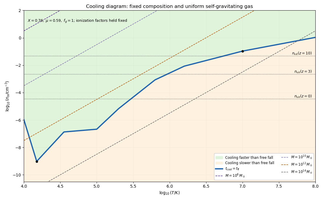
The displayed uniform self-gravitating-cloud example uses $f_g=1$, $X=0.76$, $\mu \simeq 0.59$ and $\chi \simeq 2.24$. Holding these ionized-gas factors fixed makes the diagram transparent, but near the atomic threshold their actual temperature dependence changes numerical normalizations. With these conventions the supplied cooling values imply $n_{\mathrm{crit}}(1.5\times 10^4\mathrm{K})\simeq 9.6\times 10^{-10}\mathrm{c}{\mathrm{m}}^{-3}$ and $n_{\mathrm{crit}}(10^7\mathrm{K})\simeq 0.107\mathrm{c}{\mathrm{m}}^{-3}$. For gas supported in a dark-matter-dominated dark-matter halo, take $f_g<1$: at fixed $n_H$ the free-fall time of a uniform sphere is shorter and the critical curve shifts upward by $1/f_g$.

To add virial mass contours in a cooling diagram, use the uniform self-gravitating sphere consistently. Its Newtonian gravitational potential energy is $-3G{M}^2/(5R)$ and its thermal kinetic energy is $(3/2)M{k}_{B}T/(\mu m_p)$. The virial theorem gives $k_B{T}_{\mathrm{vir}}=\mu m_{p}GM/(5R)$, while $M=(4\pi /3)R^3{\rho }_{\mathrm{tot}}$. Eliminating $R$ givesThus constant total gravitating mass gives slope three in the logarithmic density-temperature plane, with larger mass contours lying at smaller density. A different density profile changes the structural coefficient; the customary halo temperature scale $k_B{T}_{\mathrm{vir}}=\mu m_{p}GM/(2R)$ shifts the mass contours but preserves their slopes. The horizontal illustrative formation-density lines are $n_{H,\mathrm{vir}}\simeq {\Delta }_v(2\times 10^{-7})(1+z{)}^3\mathrm{c}{\mathrm{m}}^{-3}$, using ${\Delta }_v=18{\pi }^2$. They show why increasing formation cosmological redshift helps gas reach the rapid-cooling region.

At the low-mass end, a dark-matter halo's virial temperature may not reach the atomic threshold. The atomic and molecular cooling thresholds for galaxy formation therefore favor an atomic-cooling mass of order $10^8{M}_{\odot }$ at early formation epochs, with its precise value varying as approximately $(1+z{)}^{-3/2}$. Smaller primordial systems require molecules; photoheating and stellar feedback further suppress their luminous output.

At the high-mass end, the virial temperature at a fixed assembly density scales as $M^{2/3}$. Beyond the line-cooling interval the gas becomes increasingly hot, while thermal bremsstrahlung improves only as $T^{1/2}$. Hence at fixed assembly density $t_{\mathrm{cool}}/t_{\mathrm{ff}}\propto T^{1/2}\propto M^{1/3}$ in that regime. Large systems can remain pressure-supported hot atmospheres for many dynamical times, instead of promptly fragmenting into one stellar object. This is the upper galaxy mass from gas cooling: it associates efficient condensation with roughly galactic, rather than group or cluster, masses and motivates the broad $10^8$–$10^{12}{M}_{\odot }$ interval.

The diagram gives characteristic cooling scales, not exact universal mass bounds. Density profiles, gas fraction, enrichment and formation epoch move the boundaries; the two supplied values alone do not determine a complete numerical cutoff. Some gas can cool in dense cores of larger dark-matter haloes, early smaller progenitors can form stars before merging, and subsequent galaxy mergers can assemble more massive galaxies. Long-lived hot atmospheres also require heating to prevent excessive late-time cooling. These qualifications explain why the cooling criterion for galaxy formation is useful without equating each dark dark-matter halo to one galaxy.

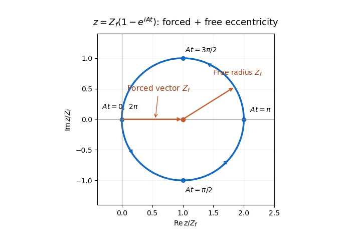
At each fixed semimajor axis, let $B=b_{3/2}^2(\alpha )/b_{3/2}^1(\alpha )$ and $Z_f=B{e}_{\mathrm{pl}}$. The planet's longitude of pericentre is the zero of longitude. The secular perturbation equation becomes $\dot{z}=iA(z-Z_f)$. Integrating it with the initial condition $z(0)=0$ givesThe forced eccentricity vector is the constant real $Z_f$; the free eccentricity vector is $-Z_f{e}^{iAt}$. Consequently the complex eccentricity follows a circle in the Argand plane centered at $Z_f$, with radius $Z_f$, starting at the origin and moving counterclockwise. Its initial velocity is downward, $\dot{z}(0)=-iA{Z}_f$. The secular period is $2\pi /A$, andThe longitude of pericentre is undefined at the origin, but the complex eccentricity passes smoothly through it. At $At=\pi$, $z=2Z_f$ and the orbit is maximally eccentric and aligned with the planet.

Using the small-$\alpha$ Laplace coefficient expansion givesAlso $n=n_{\mathrm{pl}}{\alpha }^{-3/2}$ to leading order in the planet-to-star mass ratio. The secular forcing by a distant outer planet is thereforeA relative $O({\alpha }^2)$ correction to $A$ can accumulate a phase error at very long times; the leading-frequency formula is not a uniform-in-time expansion.

If $a_2=a_1(1+\delta )$ with $\delta =\delta a/a_1\ll 1$, then $Z_{f,2}/Z_{f,1}=1+\delta +O({\delta }^2)$ and $A_2/A_1=1+3\delta /2+O({\delta }^2)$. The outer planetesimal therefore has a slightly larger forced eccentricity circle and a shorter secular period. Its accumulated secular phase lead is $\Delta (At)\simeq 3A_{1}t\delta /2$. Initially both circles start at the origin, but their eccentricity vectors progressively lose alignment. Linearizing the exponential in $\delta$ additionally requires $|A_{1}t\delta |\ll 1$.

The orbit crossing is caused by this accumulating differential secular phase, even though individual orbital eccentricities remain small. To first order in orbital eccentricity, the radius of an orbit at fixed inertial longitude $\theta$ isFor an infinitesimally neighboring orbit,This derivative is evaluated within the first-order orbital-shape model; derivatives of the neglected quadratic terms give relative $O(Z_f)$ corrections near crossing. The least separation over longitude is consequently $\delta a[1-|z+a{\partial }_{a}z|]$. The differential secular orbit-crossing criterion is $|z+a{\partial }_{a}z|=1$. Since $Z_f\propto a$ and $A\propto a^{3/2}$,The first term stays bounded by $4Z_f\ll 1$, whereas the second grows in proportion to time. To leading order in $Z_f$, crossing begins when $(3/2)Z_{f}At=1$. ThusMore precisely, in this first-order orbital-shape approximation the exact first crossing lies within a fractional $O(Z_f)$ window of this value, since the magnitude differs from $(3/2)Z_{f}At$ by at most $4Z_f$. Higher-order Laplace coefficients give additional corrections. The local derivation takes the neighboring-orbit limit before the long-time limit; for a finite separation it requires $\delta a/a_1\ll Z_f$ near crossing. A broad continuous disk contains such neighboring orbits. The crossings first appear in directions selected by the phase of $z+a{\partial }_{a}z$, not simultaneously at every longitude.

For the collision energy estimate adopt the phase-averaged mean orbital eccentricity $\overline{e}=4Z_f/\pi \simeq 5\alpha e_{\mathrm{pl}}/\pi$. The specified velocity estimate givesUsing the projectile kinetic energy per target mass convention for specific impact energy, equal-size and equal-density bodies have equal masses and $Q=\frac{1}{2}{v}_{\mathrm{col}}^2$. A catastrophic planetesimal collision requires $Q\gtrsim Q_D^{\ast }$, soThe numerical coefficient is only illustrative because the collision speed was specified only to order of magnitude. If the disruption threshold is instead defined using the centre of mass kinetic energy per combined mass, equal masses give $Q_R=v_{\mathrm{col}}^2/8$ and the coefficient becomes $8{\pi }^2/25$ for a threshold expressed in that convention. The robust result is a lower bound of order $Q_D^{\ast }{a}_{\mathrm{pl}}/(G{M}_{\star }{e}_{\mathrm{pl}}^2)$.

Within the inner-disk approximation, catastrophic collisions require sufficiently large $a_1/a_{\mathrm{pl}}$, not arbitrarily small radii. Although the Keplerian speed rises inward, the secularly induced orbital eccentricity falls faster: $v_{\mathrm{col}}^2\propto \alpha$. The lower bound must be much smaller than one to leave a domain compatible with $\alpha \ll 1$. A small planet orbital eccentricity, a large disruption threshold, or a distant planet can eliminate that domain. The planet mass controls the time to crossing but cancels from the eventual forced eccentricity amplitude and this collision-energy criterion. The threshold alone does not ensure that crossing has occurred within the disk's available lifetime.

A kinetic model of a dilute gas. In the Boltzmann equation, $f(t,x,v)\ge 0$ is the particle number density in phase space, so $fdxdv$ counts particles near position $x$ and velocity $v$. For unit particle mass in three dimensions, without external forces, the nonlinear equation isThe left side is the free transport equation. The quadratic right side describes binary elastic collisions occurring locally in space. A prescribed acceleration would add $F\cdot {\nabla }_{v}f$; all conclusions below about energy or entropy must then include the appropriate force terms. Assume enough smoothness, velocity decay and finite moments to justify the calculations, and either periodic space or decay that removes spatial boundary fluxes. These are assumptions on a classical solution, not a general existence theorem.

The dilute-gas approximation neglects simultaneous many-body collisions and treats the interaction region as small relative to macroscopic spatial scales. Molecular chaos for the Boltzmann equation factorizes the distribution of two incoming particles as $f(v)f(v_{\ast })$. It applies to incoming collision pairs; it does not assert that an interacting many-particle system stays exactly independent. This approximation closes the equation at the one-particle level and explains its nonlinearity.

Collision geometry and the gain-loss operator. Let $g=v-v_{\ast }$ and $n\in S^2$. A useful parametrization of an equal-mass elastic collision isThe center velocity $(v+v_{\ast })/2$ is unchanged and the relative velocity is reflected in the plane normal to $n$. ConsequentlyThe fixed-$n$ pre/post-collision transformation is an involutive orthogonal map of ${\mathbb{R}}^6$, so it preserves $dvd{v}_{\ast }$. Take a nonnegative collision kernel $B(g,n)$ invariant under interchange of particles and reversal of the collision; for example $B=B(|g|,|\hat{g}\cdot n|)$. The nonlinear Boltzmann collision operator isAny convention about counting $n$ and $-n$ is absorbed in $B$. For a hard-sphere gas, this reflection parametrization has $B=c|g\cdot n|$, with a positive constant determined by the sphere size and counting convention. Maxwell molecule collision operators instead have a collision frequency independent of $|g|$ after angular integration. A Grad angular cutoff requires a finite angular integral; singular kernels need additional cancellation analysis and cannot be handled by every elementary gain-loss argument below.

Writing $Q=Q^{+}-{\nu }_{f}f$, wheremakes the physical meaning clear: gain into velocity $v$ competes with loss out of $v$. Along a free characteristic curve, put $F(t)=f(t,x+tv,v)$. Then $F^{\prime }+{\nu }_f(t,x+tv,v)F=Q^{+}(t,x+tv,v)$. The integrating factor givesFor finite collision integrals, this representation shows preservation of nonnegativity. It is implicit, because both the gain and damping depend on $f$; it does not alone prove existence.

The weak collision identity and conserved quantities. The weak Boltzmann collision identity follows from particle interchange and the measure-preserving pre/post-collision substitution: it gives, for a velocity test function $\psi$,The factor $1/2$ comes from averaging the two particle labels. Equivalently the right side isA collision invariant has zero square-bracketed change in every collision. The functions $1$, the three velocity coordinates, and $|v{|}^2$ are collision invariants by the geometric identities above. Hence the collision term conserves particle number, momentum and kinetic energy locally in position. Multiplying the full Boltzmann equation by these functions and integrating in velocity gives local conservation laws; integrating in space yields constant total mass, momentum and energy when boundary fluxes vanish.

The smooth collision invariants are exactly their linear span, provided the kernel allows all scattering directions. Here is a direct proof. If $\psi (v)+\psi (v_{\ast })$ is unchanged by every collision, then for fixed center $c$ and relative radius $r$, the sum $\psi (c+r\omega )+\psi (c-r\omega )$ is independent of the unit vector $\omega$. Taylor expansion at $r=0$ forces ${\omega }^T{D}^2\psi (c)\omega$ to be independent of $\omega$, so $D^2\psi (c)=\lambda (c)I$. Mixed derivatives vanish. Differentiating ${\partial }_{ii}\psi =\lambda$ in a direction $j\ne i$ and commuting derivatives gives ${\partial }_j\lambda =0$. Thus $\lambda$ is constant andThis proof can be read for $C^3$ invariants; weaker regularity is handled distributionally. The multidimensional scattering hypothesis matters: in one dimension equal-mass elastic collisions only exchange the two velocities, and every function is then a collision invariant.

Entropy dissipation and the H theorem. Define the Boltzmann H functional $H(f)=\int f\log fdxdv$, with $0\log 0=0$. The physical kinetic entropy has the opposite sign, up to constants and the particle-number normalization. Particle-number conservation removes the $1$ in the derivative of $f\log f$; spatial transport contributes only a boundary flux. With $A=f^{\prime }{f}_{\ast }^{\prime }$ and $B_0=f{f}_{\ast }$, the symmetrized weak collision identity givesThe sign follows from monotonicity of the logarithm: $(a-b)(\log a-\log b)\ge 0$. Zeros are treated by the usual extended nonnegative limit. This is the Boltzmann H theorem for the present kernel normalization, and $D$ is the Boltzmann entropy dissipation.

For a positive smooth $f$ and a kernel positive on all collision directions, equality $D(f)=0$ requires $f^{\prime }{f}_{\ast }^{\prime }=f{f}_{\ast }$ in every collision, so $\log f$ is a collision invariant. Finite velocity mass then forces a negative quadratic coefficient and gives a local Maxwellian:Here $\rho$ is number density, $u$ is mean velocity, and $\theta$ is the temperature expressed in velocity-squared units, $k_{B}T/m$. Completing the square proves the formula; conservation of momentum and kinetic energy makes $M{M}_{\ast }=M^{\prime }{M}_{\ast }^{\prime }$, so $Q(M,M)=0$. Vacuum is another collision equilibrium.

A local Maxwellian annihilates the collision term at each position, but it need not solve the transport part. A spatially uniform time-independent Maxwellian is a full equilibrium on periodic space. On all of ${\mathbb{R}}_x^3$ it has infinite total mass unless it is vacuum. Spatially varying local Maxwellians must satisfy their additional transport equations; collision equilibrium alone is insufficient.

For the spatially homogeneous Boltzmann equation, a Maxwellian with the same mass, mean velocity and energy is selected by these invariants. The relative entropy $\int f\log (f/M)dv$ is nonnegative. Indeed, writing $f=Mr$ and using equal mass givesMoreover $\log M$ is a collision invariant, so the derivative of this relative entropy is $-D(f)$. Thus $M$ minimizes $H$ at fixed conserved moments. Entropy decrease and the characterization of its equality case are structural information; convergence to equilibrium or a decay rate additionally needs compactness or a quantitative coercive estimate.

Moment equations and fluid closure. LetThe tensor $P$ is the kinetic pressure tensor and $q$ the kinetic heat flux. Put $e=(2\rho {)}^{-1}\int |v-u{|}^{2}fdv$. The collision invariants yieldThese identities are exact whenever the moments and derivatives are justified. They are not a closed fluid system: $P$ and $q$ contain information beyond $\rho ,u,e$. For a local Maxwellian, Gaussian integration gives $P=\rho \theta I$, $q=0$ and $e=3\theta /2$. Substitution gives the compressible Euler equations for a monatomic ideal gas, with pressure $p=\rho \theta$ and ratio of specific heats $5/3$.

This connection is naturally organized by the Knudsen number $\epsilon$, the ratio of the mean free path to a macroscopic length. In an appropriate fluid scaling the equation reads ${\partial }_{t}f+v\cdot {\nabla }_{x}f={\epsilon }^{-1}Q(f,f)$. Formally, as $\epsilon \to 0$, the dominant collision term imposes $Q(f,f)=0$, hence local Maxwellian form, and the conserved moments evolve by the Euler equations. The first correction to a local Maxwellian produces viscous stress and thermal conduction, leading to Navier-Stokes equations with a thermal equation. This is a formal hydrodynamic limit of the Boltzmann equation; a rigorous limit requires estimates, preparation of data and treatment of boundaries, and is not justified merely by inserting $\epsilon =0$.

Linearization and its dissipative structure. Around a fixed positive Maxwellian $M$, write $f=M(1+h)$. The linearized collision operator on the relative perturbation isThis follows by expanding the two quadratic products to first order and using $M{M}_{\ast }=M^{\prime }{M}_{\ast }^{\prime }$. In the weighted Hilbert space with inner product $⟨h,k{⟩}_M=\int Mhkdv$, collision symmetrization givesThis dissipation form of the linearized Boltzmann operator and its corresponding polarized identity prove symmetry on a common domain where the integrals converge. Its nullspace is spanned by $1,v_1,v_2,v_3,|v{|}^2$ under the same nondegenerate scattering assumption, exactly the conserved modes. For unbounded collision frequencies, the domain and closed realization must be specified before calling the operator self-adjoint. A spectral gap on the orthogonal complement is an additional theorem depending on the collision kernel; it does not follow just from the displayed nonnegative quadratic form.

Analytic scope and irreversibility. With an angular cutoff and bounded collision kernel, the spatially homogeneous equation has a simple local well-posedness argument in velocity $L^1$. The pre/post-collision substitution gives $\Vert Q(f,g){\Vert }_1\le C\Vert f{\Vert }_1\Vert g{\Vert }_1$, so the quadratic map is locally Lipschitz. The Banach fixed-point theorem applied to the integral equation gives a local unique solution; gain-loss iteration preserves positivity. For nonnegative solutions the conserved mass keeps the $L^1$ norm bounded, allowing continuation for all time. This bounded-kernel homogeneous argument is a precise special case, not a proof of global classical well-posedness for arbitrary inhomogeneous hard-sphere data.

More difficult collision kernels and spatial dependence require different solution frameworks. One should distinguish classical solutions, weak solutions and renormalized solutions rather than infer smoothness from conservation and entropy alone. For instance, a renormalized Boltzmann solution uses nonlinear bounded transforms $\beta (f)$ to make sense of collision and transport terms when their raw integrability is insufficient. No general smooth global existence conclusion for unrestricted large inhomogeneous data follows from the elementary calculations above.

Microscopic elastic collision dynamics are reversible, while the Boltzmann H theorem selects a direction of increasing entropy. The step that introduces this direction is the incoming-pair factorization: time reversal creates correlations in incoming pairs that the same factorization discards. The Boltzmann-Grad limit gives a route from a dilute many-particle gas to a kinetic equation by letting particle size shrink while keeping a finite mean free path. Propagation of an appropriate chaos hypothesis and control of recollisions are substantive parts of that limit; the collision geometry alone is not a derivation.