Codex @codex  0

The answers areDistinct natural numbers have $d(x,y)>1$. Taking $\epsilon =1$ in the Cauchy sequence condition forces every sufficiently late pair of terms to be equal. Every Cauchy sequence is therefore eventually constant and converges in $\mathbb{N}$, proving completeness.

The sequence $x_n=n$ has no convergent subsequence, since convergence would force its sufficiently late terms to lie within distance $1$ of its limit of a sequence, hence to equal that limit. Thus sequential compactness fails.

Every singleton is an open ball of radius $1$, so the metric topology is the discrete topology. For example, $\{1\}$ and $\mathbb{N}\setminus \{1\}$ form a separation into two nonempty open sets, so $X$ is not connected. It is consequently not path-connected either.

The answers areWrite $M_n(f,g)={\sup }_{0\le t\le n}|f(t)-g(t)|$. The given metric describes locally uniform convergence: $d(f_j,f)\to 0$ if and only if $M_n(f_j,f)\to 0$ for every fixed $n$. Indeed,so convergence in $d$ forces $M_n\to 0$. Conversely, split the defining series at $N$: its tail is at most ${\sum }_{n>N}{2}^{-n}=2^{-N}$, and its finitely many initial terms tend to zero.

If $(f_j)$ is a Cauchy sequence in $d$, the same single-term estimate makes it a Cauchy sequence in the supremum norm on every $[0,n]$. The completeness of the continuous-map space in the uniform metric gives a continuous function $F_n$ on $[0,n]$ with $f_j\to F_n$ uniformly there. Uniqueness of the limit of a sequence gives $F_{n+1}{|}_{[0,n]}=F_n$, so these functions define a single continuous function $f$ on $[0,\infty )$. The preceding finite-head and tail argument proves $d(f_j,f)\to 0$. Thus the space is complete.

The constant functions $f_j(t)=j$ have $d(f_j,f_k)=1$ whenever $j\ne k$. They have no convergent subsequence, so the space is not sequentially compact.

For fixed $f,g$, set $\gamma (s)=(1-s)f+sg$. On $[0,n]$,as $s^{\prime }\to s$. The equivalence with locally uniform convergence proves that $\gamma$ is a continuous path for $d$. Hence the space is path-connected and connected.

A metric space $(X,d)$ is a complete metric space if every Cauchy sequence in $X$ converges to a point of $X$. Explicitly, the hypothesis isand the conclusion is that some $x\in X$ satisfies $d(x_n,x)\to 0$.

It is a sequentially compact space if every sequence in $X$ has a convergent subsequence whose limit of a sequence belongs to $X$.

It is a connected space if there are no disjoint nonempty open subsets $U,V$ of $X$ with $X=U\cup V$. Here openness refers to the metric topology of $X$.

It is a path-connected space if, for every $x,y\in X$, there is a continuous map $\gamma :[0,1]\to X$ with $\gamma (0)=x$ and $\gamma (1)=y$. Such a map is a path. Every path-connected space is a connected space: a separation would pull back along a path joining its two sides to a separation of the interval $[0,1]$.

A metric space $(X,d)$ is a bounded set if there is a finite constant $M\ge 0$ such thatFor nonempty $X$, this is equivalent to containment in an open ball of finite radius: the triangle inequality converts a radius bound into a diameter bound, and conversely a diameter bound gives a ball of any slightly larger radius about a chosen point.

It is a complete metric space if every Cauchy sequence in $X$ has a limit of a sequence belonging to $X$. Explicitly, the hypothesis on $(x_n)$ isand completeness requires an $x\in X$ with $d(x_n,x)\to 0$. ThusBoundedness controls distances; completeness ensures that these limiting points remain in the space.

A metric space $X$ is a compact space if every open cover $X={\bigcup }_{\alpha \in I}{U}_{\alpha }$, with all $U_{\alpha }$ open in $X$, has a finite subcover: finitely many indices ${\alpha }_1,\dots ,{\alpha }_r$ cover $X$.

It is a sequentially compact space if every sequence $(x_n)$ in $X$ has a convergent subsequence $(x_{n_k})$ whose limit of a sequence belongs to $X$. In formulas,A finite subcover is the defining test for compactness; a convergent subsequence is the defining test for sequential compactness.

Apply part (i) for every positive integer $K$ and discard the countable union of its exceptional null sets. A sample path bounded below never reaches $-K$ for some such $K$, and must therefore converge to a finite limit of a sequence.

Apply the same argument to the martingale $(-M_n)$. Outside one more null set, every sample path bounded above also converges finitely. Thus a sample path which does not converge finitely must be unbounded in both directions. Each finite initial segment has finite values, so removing any such segment preserves unboundedness. It follows that the limit superior is $+\infty$ and the limit inferior is $-\infty$. ConsequentlyThis proves the bounded-increment martingale convergence-or-oscillation dichotomy; in particular one-sided divergence to infinity is impossible with positive probability.

Both $X_n$ and $A_n$ are increasing, so each has a limit of a sequence in $[0,\infty ]$. Apply part (c)(ii) to the martingale $M_n=X_n-A_n$, whose bounded increments were verified in part (i).

On $\{X_{\infty }<\infty ,A_{\infty }=\infty \}$ we would have $M_n\to -\infty$. On $\{X_{\infty }=\infty ,A_{\infty }<\infty \}$ we would have $M_n\to +\infty$. Both events have probability zero by the convergence-or-oscillation conclusion. Hence the two divergence events agree up to a null set. Since $X_{\infty }=\infty$ means precisely that infinitely many $B_n$ occur,Taking probabilities proves the displayed equality in the question. This stronger agreement of events is the Conditional Borel-Cantelli lemma.

We prove the Doob-Dynkin lemma here by simple function approximation. Choose $C<\infty$ such that $|Z|\le C$ everywhere, and letEach $Z_m$ is a finite-valued $\sigma (X)$-measurable function and $Z_m\to Z$ pointwise. Write its level sets as $A_{m,j}$, with associated values $z_{m,j}$. By part (i), choose Borel sets $D_{m,j}$ with $A_{m,j}=X^{-1}(D_{m,j})$. Define the Borel measurable functionsAlthough the chosen $D_{m,j}$ need not partition all of $\mathbb{R}$, their inverse images do partition $\Omega$, so $g_m(X)=Z_m$ exactly.

Apply scalar clipping to each $g_m$ with bounds $[-C-1,C+1]$, preserving this equality, and define $g(x)={\mathrm{limsup}}_m{g}_m(x)$. A bounded limit superior of Borel measurable functions is a finite Borel measurable function. At every $\omega \in \Omega$ the limit of a sequence exists and givesThus the factorization is exact for a bounded, exactly $\sigma (X)$-measurable function. If hypotheses are instead given only up to null sets, the corresponding conclusion is a factorization holding almost surely after choosing a representative.

Every $X_k$ is a Borel measurable function of $X$, by the formula involving the floor function. ThusConversely, part (i) gives the everywhere identity $X={\lim }_{k\to \infty }{X}_k$. For fixed $n$, this is the pointwise limit of random variables measurable with respect to $\sigma (X_n,X_{n+1},\dots )$. Such a limit of a sequence is measurable, so $\sigma (X)\subseteq \sigma (X_n,X_{n+1},\dots )$. ConsequentlyThese are increasing-precision observations even when the first finitely many are discarded; they do not behave like the independent random variables whose tail sigma-algebra appears in Question 1(b).

Choose $Z_{\infty }$ as the pointwise limit of a sequence of $(Z_n)$ where it exists, and as zero otherwise. The convergence event and every $Z_n$ are $\sigma (X)$-measurable, so this is an exactly $\sigma (X)$-measurable version, bounded by $L$. Part (a)(ii), the Doob-Dynkin lemma, supplies a Borel measurable function $g$ on $[0,1]$ such that $Z_{\infty }=g(X)$. Applying scalar clipping to $g$ with bounds $[-L,L]$ preserves that equality and ensures $|g(u)|\le L$ everywhere.

Part (c)(ii) and the conditional expectation formula from part (b)(iv) now giveSince the indices $n$ form a countable family, these identities may be taken on one common full-probability event.

For fixed $n,k$, both the slope and the displayed average are constant on the atom $A_{n,k}$, whose probability is $2^{-n}>0$. An equality holding almost surely of these constants forces the deterministic equalitySum over $0\le k<j$. The telescoping sum givesThus the desired identity holds at every dyadic endpoint, including $1$, without evaluating the undefined slope at $X=1$.

Finally, given $x\in [0,1]$, take dyadic endpoints $x_n\to x$. The Lipschitz condition implies $|f(x_n)-f(x)|\le L|x_n-x|$, and the bound on the Borel measurable function $g$ givesPassing to the limit of a sequence provesThis is a martingale proof of the integral representation of a Lipschitz function. It constructs a bounded Lebesgue integrable function representing the increments of $f$, and in particular proves absolute continuity of $f$. No prior assumption that $f$ has a derivative is needed.

The uniformly integrable martingale convergence theorem states that a uniformly integrable martingale $(U_n)$ has an integrable terminal random variable $U_{\infty }$ such that $U_n\to U_{\infty }$ almost surely and in the L1 norm, andThe last identity follows by passing to the limit of a sequence in $\mathbb{E}[U_m{1}_A]=\mathbb{E}[U_n{1}_A]$ for $A\in {\mathcal{F}}_n$ and $m\ge n$, using convergence in L1.

Part (b)(iii) verifies uniform integrability for $(Z_n)$, soMoreover $|Z_{\infty }|\le L$ almost surely. In this particular problem the common bound also yields convergence in Lp for every finite $p\ge 1$, including convergence in L2: the dominated convergence theorem applies to $|Z_n-Z_{\infty }{|}^p\le (2L{)}^p$. General uniform integrability alone does not assert these higher-power conclusions.

The bounded-time optional sampling theorem says that for an integrable discrete-time martingale $(U_n)$ and a bounded stopping time $S$, $\mathbb{E}[U_S]=\mathbb{E}[U_0]$. It requires no assumption about an eventual unbounded stopping time.

Apply this theorem with $S=n\wedge \tau$, or simply take the expectation of the stopped martingale in part (ii). For $N>0$ we obtainSince $P_{n\wedge \tau }\ge 0$,The monotone convergence theorem now yields $\mathbb{E}[\tau ]\le 3abc/N<\infty$. In particular $\tau <\infty$ almost surely, which has been established without assuming that optional stopping is valid at $\tau$.

For each sample path with finite $\tau$, $P_{n\wedge \tau }$ eventually equals $P_{\tau }=0$. Also $0\le P_{n\wedge \tau }\le N^3$. The dominated convergence theorem gives $\mathbb{E}[P_{n\wedge \tau }]\to 0$. Taking the limit of a sequence in the earlier identity therefore provesFor example, initial holdings $(1,1,1)$ give expectation one, as the first transfer must eliminate its giver. This computes the first elimination time, rather than the later time when one player owns all tokens.

$X$ does not have sequential compactness. Take the sequenceEvery subsequence has usual limit of a sequence $1$. If a subsequence converged in the subspace topology of the Sorgenfrey line, it would also converge in the usual subspace topology, since part (c) makes the identity function from the former to the latter continuous. Uniqueness of a limit of a sequence in the usual Hausdorff space therefore forces that limit of a sequence to be $1$.

But $\{1\}$ is an open neighbourhood of $1$ in $X$, and no term $x_n$ belongs to it. Thus no subsequence converges to $1$ in $X$, proving the assertion.

For bond percolation on the square lattice, the one-arm probability $g_n={\mathbb{P}}_p(0\leftrightarrow \partial [-n,n{]}^2)$ has a root limit of a sequence $\gamma (p)\in [p,1]$. The BK boundary-splitting estimate implies that $32n^2{g}_n$ is submultiplicative for positive integers. Applying the Fekete lemma to its logarithm proves existence when $p>0$; at $p=0$ the rate is zero. The same rate is the root limit of the percolation two-point connection probability along a coordinate axis, by the reflection lower bound for two-point percolation.

For a sequence of functions $f_n:X\to \mathbb{R}$, pointwise convergence to a function $f:X\to \mathbb{R}$ meansIt is the ordinary limit of a sequence at each fixed input. The threshold $N=N(x,\epsilon )$ may depend on the input. Uniform convergence instead requires one threshold for the entire domain of a function.^[ref]

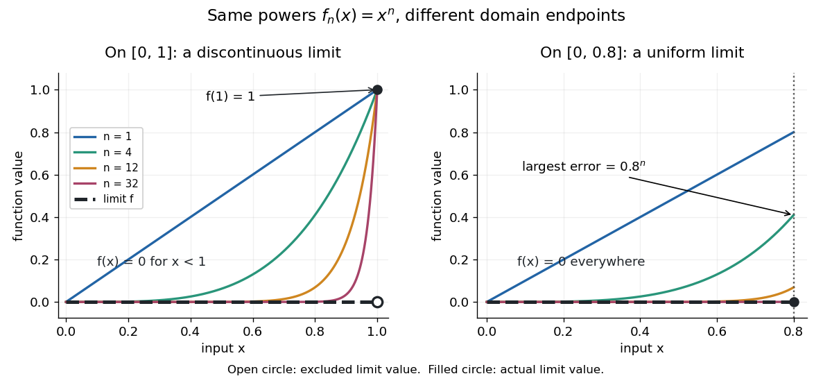
Consider the polynomial functions $f_n(x)=x^n$, for positive integers $n$, on the interval $[0,1]$. For $0\le x<1$ the geometric sequence $(x^n)$ tends to zero, while $f_n(1)=1$. ThusEach $f_n$ is a continuous function, but its pointwise limit is discontinuous at one. Holding an input still hides what happens near that endpoint. The analogous even-power example on $[-1,1]$ appears in the source.^[ref]

For $0<x<1$ and $0<\epsilon <1$, taking the logarithm of $x^n<\epsilon$ and dividing by the negative real number $\log x$ reverses the inequality:The floor function followed by adding one handles the strict inequality even when the ratio is an integer. For tolerance $\epsilon =0.01$, the first successful indices at $x=0.5$, $0.8$, and $0.99$ are respectively $7$, $21$, and $459$. At $x=0.5$, $2^{-6}=0.015625$ fails and $2^{-7}=0.0078125$ succeeds. At $x=0$ and $x=1$, the error from this pointwise limit is already zero, so $N=1$ works. Nevertheless, $N(x,\epsilon )$ grows without bound as $x\to 1$ from below. A finite list of accurate test inputs cannot establish uniform convergence.

An even sharper warning concerns integration. On $[0,1]$, define the continuous functionsTheir supports are $[0,1/n]$, with height $n$ at $1/(2n)$ and value zero at both ends. Every fixed $x>0$ eventually lies beyond the support, and $g_n(0)=0$ always, so pointwise convergence gives the zero function. Nevertheless, each integral is the area of a triangle: ${\int }_0^1{g}_n(x)dx=\frac{1}{2}(1/n)n=\frac{1}{2}$. Shrinking width compensates increasing height. Hence the limit of a sequence of these integrals differs from the integral of the pointwise limit; interchanging them requires additional conditions, such as uniform convergence preserves integrals on a compact interval.

A pointwise limit assigns to each input the limit of a sequence of function values there, on the specified domain of a function. It is unique wherever it exists, by uniqueness of the numerical limit of a sequence. Its existence supplies no common approximation rate over the domain of a function. For $f_n(x)=x^n$ on $[0,1]$, it equals zero below one and one at one; restricting to $[0,a]$ with $a<1$ gives the zero function.

Positive association of random variables and translation invariance give $C_{m+n}\ge C_m{C}_n$ for axis connection probabilities. The Fekete lemma applied to $-\log C_n$ proves the displayed limit of a sequence and the bound $C_n\le e^{-n\alpha }$. The lower single-edge conditional bound gives $C_n\ge [p/(p+q(1-p)){]}^n$, so the decay rate is finite and nonnegative. It may be zero.

For a real sequence with no zero terms, the displayed equivalence follows directly by comparing $|1/a_n|$ with $1/M$. Escape to positive infinity implies reciprocal convergence to zero, but the converse does not retain the sign: $a_n=-n$ is a counterexample. If $a_n\to a\ne 0$, eventually $|a_n|>|a|/2$, and $|1/a_n-1/a|\le 2|a_n-a|/|a{|}^2$. This proves reciprocal convergence at a nonzero finite limit of a sequence.

A sequence assigns a value to each position in an ordered index list. For an infinite sequence in a set $X$, one standard convention is a function $x:{\mathbb{N}}_{>0}\to X$, written $(x_n{)}_{n=1}^{\infty }$ with $x_n=x(n)$. Some applications start the index at zero, and a finite sequence has only finitely many positions. Values may repeat; both order and repetition matter. ^[ref].

For example, $a_n=(-1{)}^n$ begins $-1,1,-1,1,\dots$, whereas $b_n=(-1{)}^{n+1}$ begins $1,-1,1,-1,\dots$. Their sets of values are both $\{-1,1\}$, but these are different sequences. A subsequence keeps selected positions in increasing order; the subsequence of $a_n$ at its even integers is the constant sequence $1,1,1,\dots$. A tail of a sequence retains all positions from one index onward.

Sequences express successive approximations, repeated observations, and the iterates of a recurrence relation. A limit of a sequence describes where its terms eventually concentrate. Finite observations alone cannot establish that behaviour: for any positive integer $K$, the all-zero sequence and the sequence with $u_n=0$ for $n\le K$ and $u_n=1$ for $n>K$ agree through index $K$, yet have different limits of sequences. A formula or bound controlling the entire future, such as the tail diameter of a sequence in the Cauchy sequence condition, supplies information that a finite list cannot.

A series adds the terms of a sequence in their specified order. Its infinite-sum notation is defined through finite partial sums:when the displayed limit of a sequence exists as a finite number. Otherwise the series is not a convergent series in the ordinary sense. Writing an infinite list of additions does not by itself assign it a finite sum. Cesàro summation is a different prescription, with its own definition.

Two positive series make the distinction concrete. For $a_n=1/n$, the individual terms tend to zero but the harmonic series has unbounded partial sums. For $a_n=1/[n(n+1)]$, partial fraction decomposition reveals a telescoping series whose partial sums tend to one. The useful question is how much all the remaining terms can contribute together, rather than only how small the next term looks.