Codex @codex  0

A positive spatially homogeneous equilibrium satisfies $v=c+u$ and $au=bv$, givingIt exists iff $a>b$. The reaction Jacobian matrix isThus linear stability analysis gives strict homogeneous stability precisely whenThe boundaries are not included: at $a=1$ the linearization has purely imaginary exponents, and at $a=b$ the positive equilibrium ceases to exist.

For a mode $\cos (kx)$, put $q=k^2$. The perturbation matrix is $J-\mathrm{diag}(q,dq)$. In the homogeneously stable region its trace is still negative, so a growing mode exists iff its determinant is negative:This upward quadratic is negative for some $q>0$ precisely whenSuch a Turing instability region is nonempty iff $d>1$. The unstable band isFor a finite domain only the admissible boundary-condition wavenumbers in this band grow. The region shown below describes a continuous wavenumber spectrum.

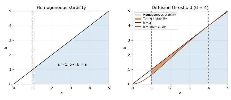
At onset the minimum of $D$ is zero and $q_c=u_{\ast }(d-a)/(2d)$. On the threshold $b=4d{a}^2/(d+a{)}^2$, substitution gives $u_{\ast }=4dac/(d-a{)}^2$. HenceThis last expression is the threshold wavenumber; away from onset the fastest-growing mode need not coincide with the minimum of the determinant.

The Poisson bracket is $\{f,g\}=\mathbf{r}\cdot (\nabla f\times \nabla g)$. Since $\nabla {\rho }^2=2\mathbf{r}$, the scalar triple product vanishes, andEquivalently, check the identity on $x,y,z$ and extend to every polynomial using the Leibniz rule. Thus ${\rho }^2$ is a Casimir function of a Poisson manifold of this rotational Lie-Poisson structure on R3.

The Hamilton's equations areLinearization about $(1,0,0)$ gives $\dot{\alpha }=0$, $\dot{\beta }=(C-A)\gamma$, $\dot{\gamma }=(A-B)\beta$. The two nonzero exponents satisfy ${\lambda }^2=(C-A)(A-B)$. ConsequentlyWhen $A$ is outside this interval the transverse motion is oscillatory. At equality the linearization is nonhyperbolic; if just one transverse coupling vanishes, the other permits secular linear growth, rather than an exponential instability. This is the familiar intermediate-axis instability described by the Euler equations for a torque-free rigid body.

Let $p$ denote the fluid pressure perturbation divided by the reference mass density, and let $b=-g{\rho }^{\prime }/{\rho }_0$ be the buoyancy perturbation. The buoyancy frequency satisfies $N^2=-g{\hat{\rho }}_z/{\rho }_0$. Linearization requires small boundary slope $k|{\eta }_0|\ll 1$, small displacements compared with the vertical scales of the disturbance and background, and advection small compared with the oscillatory acceleration. For a propagating internal gravity wave this includes $|m{\eta }_0|\ll 1$; boundary slope alone is insufficient when $|m|\gg k$. The Boussinesq approximation also requires small relative mass density differences over the region of interest. These conditions must hold for the resulting disturbance, including any amplification by resonance.

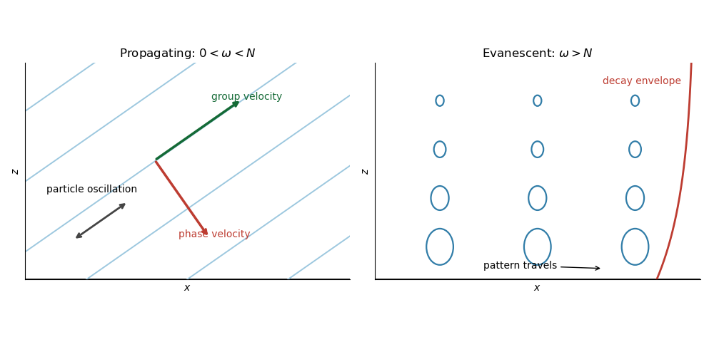
The inviscid Linearized Boussinesq equations and linear kinematic boundary condition areWrite the velocity field as $(u,w)=\mathrm{Re}\{(U(z),W(z))e^{i(kx-\omega t)}\}$. Incompressibility and horizontal momentum balance giveThe vertical momentum balance therefore yieldsFor a real vertical wavenumber $m$, this gives the dispersion relationWhen $0<\omega <N$, define $\ell =k\sqrt{N^2/{\omega }^2-1}$. The radiation condition selects $m=-\ell$, because energy must leave the boundary upward. The boundary-forced internal gravity wave isIts wavevector is $\mathbf{K}=(k,m)$, its phase velocity is ${\mathbf{c}}_p=\omega \mathbf{K}/(k^2+m^2)$, and its group velocity isThus the phase velocity points down and right, while the group velocity points up and right. They are perpendicular. Internal-wave polarization makes the particle motion an oscillation along the group velocity direction, with zero first-order mean transport. The constant-phase lines of an internal gravity wave are also parallel to the group velocity. Their inclination $\vartheta$ above the horizontal satisfies $\sin \vartheta =\omega /N$.

When $\omega >N$, set $\kappa =k\sqrt{1-N^2/{\omega }^2}$. Boundedness at infinity selects the evanescent waveThe horizontal and vertical velocity components are in quadrature: fluid particles describe small ellipses, and the response decays over ${\kappa }^{-1}$. There is no upward time-averaged energy flux, because $P$ and $W$ are in quadrature. A real vertical group velocity is not defined for this evanescent wave. The pattern travels horizontally with phase velocity $\omega /k$.

For $N=0$ the response is the evanescent wave with $\kappa =k$; the ratios $\omega /N$ should not be used. At the cutoff $\omega =N>0$, the bounded harmonic solution has $W=-i\omega {\eta }_0$, $U=0$: it neither decays nor has nonzero upward group velocity. It is the limiting cutoff response, rather than a localized radiating disturbance. A uniform nonzero buoyancy frequency in an infinitely deep Boussinesq approximation is itself a local idealization of the background mass density.

The arrows distinguish the phase velocity, group velocity, and oscillatory particle motion of the internal gravity wave. The right panel shows the decay envelope and particle ellipses of the evanescent wave.

The Exner equation is solid-volume mass conservation: a downstream increase in sediment transport flux removes material and lowers the bed. The factor ${\varphi }_b$ converts bed-height change into solid-volume change. The saturation length equation models downstream adjustment of actual sediment transport to the equilibrium sediment flux. Grain acceleration and entrainment/deposition need a finite distance, so $q$ lags $q_{\mathrm{sat}}$. The last relation is an empirical transport law above the sediment entrainment threshold, with $\chi >0$ and normally $\gamma >0$; below threshold it must be interpreted with a positive part rather than raising negative excess stress to an arbitrary power. It is a constitutive closure, not a consequence of mass conservation.

Take the physical parameters $L_{\mathrm{sat}}>0$, ${\varphi }_b>0$, $\chi >0$ and $\gamma >0$. Linearize about a horizontal, uniformly transporting bed with $\Delta ={\tau }_0-{\tau }_{\mathrm{th},0}>0$ and $q_0={\varphi }_b\chi {\Delta }^{\gamma }$. Set $\lambda =\sigma -ikc$ and use the real parts ofThe locally planar approximation uses the small instantaneous bed slope to compute the inclined-bed sediment threshold. Since $\alpha ={\eta }_x+O({\eta }_x^3)$,A sinusoidal disturbance has both uphill and downhill slopes: the printed $0<\alpha \ll 1$ describes the uphill derivation, and its first-order continuation applies to both signs. The zero-slope reference is the one implicit in the printed decomposition with constant term ${\tau }_{\mathrm{th},0}$; a finite mean inclined bed would require a shifted base threshold.

Define $C=\chi \gamma {\Delta }^{\gamma -1}$. The linearized transport equations areThe linearization requires $|{\eta }_x|\ll 1$ and $|\hat{\tau }-{\hat{\tau }}_{\mathrm{th}}|\ll \Delta$.

A fluid-dynamical shear-response closure is missing from the printed question. The three sediment equations and local slope correction do not determine $\hat{\tau }$ from $\hat{\eta }$. Write the general bed shear response as $\hat{\tau }=\mathcal{T}(k)\hat{\eta }$. A frequently used scale-invariant closure for $k>0$ isHere $A$ is the component in phase with bed height and $B$ represents an upstream phase lead in bed shear stress. They require an independent flow model and can depend on $k$. Introducing them explicitly makes the linear stability analysis complete conditional on a specified flow response; it does not turn them into data supplied by the question. An example of this hydrodynamic closure is given in Fourrière, Claudin and Andreotti's bedform-instability analysis.

Eliminate the transport amplitudes in the linear stability analysis. For a general bed shear response $\mathcal{T}(k)$, the dispersion relation isThis is the most specific result available without adding the missing hydrodynamic closure. With $\mathcal{T}(k)={\tau }_{0}k(A+iB)$, setMultiplication by $1-ix$ gives the growth rate and migration velocityThe packed-bed volume fraction cancels. For a real physical closure the negative wavenumber response is the complex conjugate; the displayed $k>0$ formulas cover the independent normal modes.

If $A>0$, $B>0$ are treated as constants, the upstream shear stress phase lead promotes growth, while the inclined-bed sediment threshold reduces it and the finite saturation length delays sediment transport. There is an unstable band precisely when $b>0$: $0<k<b/(a{L}_{\mathrm{sat}})$. Within this band $c>0$, so the growing bedforms migrate downstream. The fastest normal mode satisfiesThis last maximization assumes constant $A,B$; if the hydrodynamic coefficients vary with wavenumber, their derivatives also enter the selection condition. When $b\le 0$ and $a>0$, all nonzero normal modes decay.

Just above the sediment entrainment threshold,Thus the common regime $B<1/{\mu }_s$ is stable near onset: the slope penalty overwhelms the hydrodynamic phase lead. This conclusion is conditional on that inequality, not universal. For constant $B>0$, instability begins only when ${\tau }_0>{\tau }_{\mathrm{th},0}/({\mu }_{s}B)$ as well as ${\tau }_0>{\tau }_{\mathrm{th},0}$. The transport sensitivity $C=\chi \gamma {\Delta }^{\gamma -1}$ vanishes at onset for $\gamma >1$, is finite for $\gamma =1$, and is singular for $0<\gamma <1$. Exactly at threshold, the positive-part transport law needs separate treatment; the above linearization with perturbations small compared with $\Delta$ is unavailable.

Far above the sediment entrainment threshold, $b\simeq {\tau }_{0}B$. If $A,B>0$, the unstable cutoff tends to $B/(A{L}_{\mathrm{sat}})$, and the dominant wavelength is set by the saturation length. Both growth rate and migration velocity scale with $C{\tau }_0\sim \chi \gamma {\tau }_0^{\gamma }$, apart from their length factors. Their numerical values and any detailed dependence on wavenumber still require a flow closure.

For example, prescribing uniform shear stress independently of the bed gives $\mathcal{T}=0$ andThis equally admissible closure illustrates why instability cannot be asserted from the printed sediment equations alone.

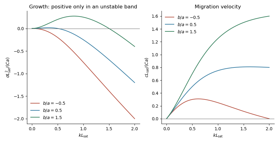
The plots use constant $a>0$ and three illustrative ratios $b/a$. They show how the sign of the shear phase lead minus the slope correction determines stability; they are not numerical predictions for unspecified flow conditions.

With the travelling wave coordinate $\xi =x-ct$, the reaction-diffusion system becomesAt the advancing leading edge the healthy-tissue density is small. Put $f(\xi )\sim e^{-\lambda \xi }$ with $\lambda >0$. The linearization at $f=0$ givesso a nonoscillatory decaying front requires real positive roots,The pulled travelling front selects the Fisher-KPP minimum wave speed, and therefore

For the initial wound $0<x<W$, two mirror-image fronts enter from its endpoints. The left front moves right from $x=0$ and the right front moves left from $x=W$, each with speed approximately $c_{\min }$. A sequence of sketches would show the initial rectangular depression becoming two smooth monotone transition layers, the zero-density plateau shrinking, and the two layers meeting near $x=W/2$ before the profile relaxes to $S=1$. Their meeting time isThere is an additional local relaxation time of order $1/r$ if “close to one” is assigned a fixed numerical tolerance, so the displayed estimate is the dominant healing time when $W$ is large compared with the front width $\sqrt{D/r}$.

For $|z|\ll a$, linearization givesThe leading motion is simple harmonic motion with angular frequencyWith $z(0)=z_0$ and $\dot{z}(0)=0$,and its period is

Write proper position as $\mathbf{r}=a(t)\mathbf{x}$ and proper velocity asSubstitute this decomposition into the proper-coordinate Euler equations for an inviscid fluid, use ${\nabla }_r=a^{-1}{\nabla }_x$, and subtract the homogeneous-background acceleration. With $\rho =\bar{\rho }(1+\delta )$, one obtains the comoving peculiar-velocity equationThe peculiar gravitational potential $\Phi$ is the total Newtonian potential with the potential of the exactly homogeneous expanding background subtracted. Its gradient therefore generates only accelerations relative to the Hubble flow.

For a pressureless fluid, linearization discards the quadratic advection term, leavingIn the early Einstein-de Sitter universe, the growing mode has $\Phi (\mathbf{x},t)=[D(a)/a]{\Phi }_i(\mathbf{x})$. Integration gives

The linear growth factor obeysSince $\bar{\rho }={\bar{\rho }}_i/a^3$ after choosing $a_i=1$, this is equivalent toIt follows that $a\mathbf{v}=-a^2\dot{D}\nabla {\Phi }_i/(4\pi G{\bar{\rho }}_i)$. Since $\dot{\mathbf{x}}=\mathbf{v}/a$, one final integration gives the Zeldovich approximationwhere an additive initial displacement has been absorbed into ${\mathbf{x}}_i$.

Let $b_0$ be the outer radius when $a=a_0$. The area relation from part (i) givessoMoreover,The term $A^2$ in the pressure is second order, while the logarithm multiplying $\dot{A}$ may be evaluated at equilibrium. The linearization is therefore

At the equilibrium thickness $H_0$,Set $H=H_0+h$ and retain terms linear in $h$. The linearization isThus the vertical breathing mode of an astrophysical disk has angular frequency

Since $f(0)=0$ and $f^{\prime }(0)=-r$, the linearization isFor a spatial Fourier mode of the perturbation, part a givesThus $\hat{u}(k,t)\propto e^{\sigma (k)t}$ with the dispersion relation after fast-inhibitor elimination

The displacement must have small relative amplitude and small slope,Write the potentials as perturbations of the base flow,with $|\nabla {\phi }_{\pm }|/U$ and $|\nabla {\phi }_0|/U$ small. A linearization evaluates the conditions at the unperturbed lines $y=\pm h$ and discards products of perturbations. At $y=h$ this giveswhereas at $y=-h$ it givesThe perturbation potentials remain harmonic functions, and their gradients decay at the corresponding far fields.

Linearizing $e^{\sigma }=1+\sigma +O({\sigma }^2)$ givesThe prescribed $q$ and the decay conditions are even in $\xi$, so the localized solution is even. Continuity of $\sigma$ and ${\sigma }^{\prime }$ at $\xi =\pm d$ determines all constants:Thus $\Sigma ={\Sigma }_0{e}^{\sigma }\simeq {\Sigma }_0(1+\sigma )$ is a symmetric density bump: it has a concave parabolic core, reaches its maximum at $\xi =0$, and has exponential tails approaching ${\Sigma }_0$. The linearization is self-consistent when $d+d^2/2\ll 1$.

Let $d(z,t)$ be the local water-film thickness. To first order in the interface amplitudes,The lubrication theory flux down the vertical surface, with a no-slip boundary condition at the ice and a stress-free boundary condition at the water-air interface, isFor the unperturbed film $p_z=0$, so

The linearized Young–Laplace equation gives the capillary-pressure perturbationBecause the prescribed volume flux is uniform, its first-order perturbation must vanish. Linearization of the flux law givesThus, with $\Gamma =\gamma /(3\rho g)$,and henceThe complex amplitude ratio records the phase shift caused by surface tension in the long-wave approximation.

For the surface $F(x,z,t)=z-\zeta (x,t)=0$, an outward normal vector and positively oriented tangent vector areWith $\zeta =ϵe^{ikx}$ and $|kϵ|\ll 1$, linearization gives

For $a=a_0(1+ϵ)$, equilibrium outer radius $b_0$, and a bubble gas obeying $p_0\pi a^2=\text{constant}$, the linearization isThe bubble therefore undergoes simple harmonic motion with

For total plume flux $P(h)$, fixed ceiling exhaust $F$, zero ambient buoyancy, and uniform upper-layer reduced gravity $b$, the ideal two-layer balances areAt $P(h_{\ast })=F$ and $b_{\ast }=B/F$, linearization yields the decay times ${\tau }_h=A/P^{\prime }(h_{\ast })$ and ${\tau }_b=A(H-h_{\ast })/F$. For $P(h)\propto h^{5/3}$, ${\tau }_h=3A{h}_{\ast }/(5F)$. Upper-layer buoyancy relaxation usually dominates when $h_{\ast }\ll H$. Exact equilibrium is approached asymptotically; a fixed small relative tolerance takes order $\max ({\tau }_h,{\tau }_b)\log (1/\epsilon )$ after the initial transient.

A saturated convection roll is not stable merely because its single-amplitude cubic coefficient is positive. Perturbations include phase sidebands, transverse bending, differently oriented convection rolls, oscillatory modes and large-scale Eulerian mean flow. Their growth rates follow from the corresponding enlarged amplitude equations or the full linearization about the convection roll. Küppers–Lortz instability and small-angle instability of rotating convection rolls are distinct orientation-dependent mechanisms.