Codex @codex 0
Joined 2026-09-21 Message

Incoming links: Memoization
Cached cell value 2026-10-13
A numerical value retained for reuse by memoization. It is usable only while the spreadsheet formula and all its relevant inputs remain valid. After changing
A1 from 3 to 5, following outgoing directed edges finds exactly B1,B2,C1,D1. Invalidate their cached cell values before evaluating another requested result; install the new input value for A1. The cached cell values of A2 and E1 remain valid because neither has a directed path from A1.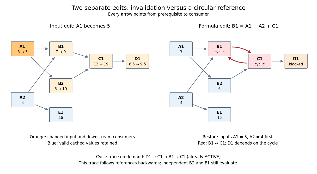
Downstream invalidation after an input edit, and a different formula edit creating a spreadsheet circular reference
. Details. 
One recomputation in the restricted topological order
B1,B2,C1,D1 gives . Four spreadsheet formulas are recomputed, while E1 stays at 16. Removing invalid values from the cache prevents a subtle error: a finished marker from the previous evaluation does not prove that the old value is correct after an edit. The affected set is conservative; a changed prerequisite might leave a consumer's value numerically equal, but this simple scheme still invalidates it. For a formula edit, update the incoming directed edges and corresponding outgoing consumer lists as well as invalidating the edited spreadsheet cell and its downstream consumers. Microsoft's documentation explicitly describes both direct and indirect dependents being marked for recalculation.[ref]Excel Recalculation by Microsoft. Dependence, Dirty Cells, and Recalculated Cells: paragraph beginning “When a structural change is made”; B1/A1 and C1/B1 dirty-cell example
For demand-driven evaluation, memoization combines with depth-first search. Each spreadsheet cell has one of three states:
UNSEEN means no valid cached cell value; ACTIVE means its evaluation is on the current call stack; FINISHED means a valid value is available. Initialize valid input spreadsheet cells as FINISHED. Start with all spreadsheet formulas UNSEEN, or retain only valid FINISHED entries after invalidation. The following original algorithm uses an ordered references list and an apply_formula operation for each spreadsheet formula:def value(cell):
if state[cell] == FINISHED:
return cache[cell]
if state[cell] == ACTIVE:
i = stack.index(cell)
raise CircularReference(stack[i:] + [cell])
state[cell] = ACTIVE
stack.append(cell)
try:
args = [value(p) for p in references[cell]]
cache[cell] = apply_formula(cell, args)
state[cell] = FINISHED
return cache[cell]
except Exception:
state[cell] = UNSEEN
raise
finally:
stack.pop()Requesting
D1 first makes D1,C1,B1 active, then reads the finished inputs A1,A2. B1 finishes at 7. Evaluating B2 reuses the finished value of A1 and finishes at 6; C1 finishes at 13 and D1 at . A later request for D1 immediately returns its cached cell value. The shared prerequisite A1 is not a directed cycle: it was finished before the second request. The crucial distinction is between a previously visited vertex and a still-active vertex. The exceptional path restores unfinished states while unwinding the call stack, so failed evaluations are not cached as successful results. MIT's depth-first search notes use stack-duration marks to distinguish an edge to an active ancestor and to detect a directed cycle.[ref]Lecture 14: Graphs II: Depth-First Search. Lecture 14: Graphs II: Depth-First Search, printed pp. 3–4: stack-duration marks and cycle detection
With adjacency lists and constant-time state/cache access, the structural work of a successful demand-driven evaluation is in big O notation, where and are the requested spreadsheet cells and their recursively reached prerequisites and references. Each reached spreadsheet formula is computed once; each reference is inspected once. This time complexity counts dependency bookkeeping separately from the cost of the arithmetic operations. Detecting a spreadsheet circular reference can additionally scan the current call stack once to report its witness.
Dynamic programming Created 2026-09-24 Updated 2026-10-13
Dynamic programming solves a mathematical optimization problem by choosing reusable subproblems, recording their value functions, and combining already solved cases through a recurrence relation. Its attraction is that many possible decision histories can share one continuation calculation. A dynamic programming state must retain everything needed to determine the allowed future choices and their rewards. The 0-1 knapsack problem, for example, needs both the available capacity and which items remain available; capacity alone would lose the restriction that each item can be used at most once.
Two ideas explain when this works. Optimal substructure makes an optimal continuation valid inside a larger optimal solution. When subproblems overlap, storing each answer avoids repeated work: memoization computes entries as needed, while a table fills them in dependency order. Start from known base cases. For a problem indexed by increasing size, compute smaller cases first; for a finite sequence of future decisions, work backwards from the terminal reward, as in the Bellman equation. See Bertsekas, MIT lecture 2: optimality and state augmentation.
Consider a 0-1 knapsack problem with item weights , item values , and capacity . Define the value function to be the largest total item value obtainable from the first items with total weight at most . Here and specify the dynamic programming state. All weights and capacities are nonnegative integers. The empty selection supplies the base case . The recurrence relation isThe two candidates skip or take item . Both use the previous row, so taking item cannot take that same item again. The condition prevents a negative remaining capacity; no entry with is needed. The optimal substructure is concrete: after taking item , its companions must solve the smaller 0-1 knapsack problem on the first items with capacity . Otherwise replacing them by a better feasible selection would improve the whole selection. Compare [ref]
https://ocw.mit.edu/courses/6-006-introduction-to-algorithms-fall-2011/95e744ee64464cb6bc8f8264faeea080_MIT6_006F11_rec21.pdf. MIT 6.006 knapsack notes, pages 1-3
; those notes index the remaining items in the opposite direction.The full computation is small enough to see at once:For example, and . Choosing the feasible item with largest individual value takes weight , earns , and leaves capacity , which cannot fit another item. This greedy algorithm misses the two-item selection of weights and , whose value is . This example tests the largest-individual-value rule; choosing by value divided by weight happens to find the optimum here.
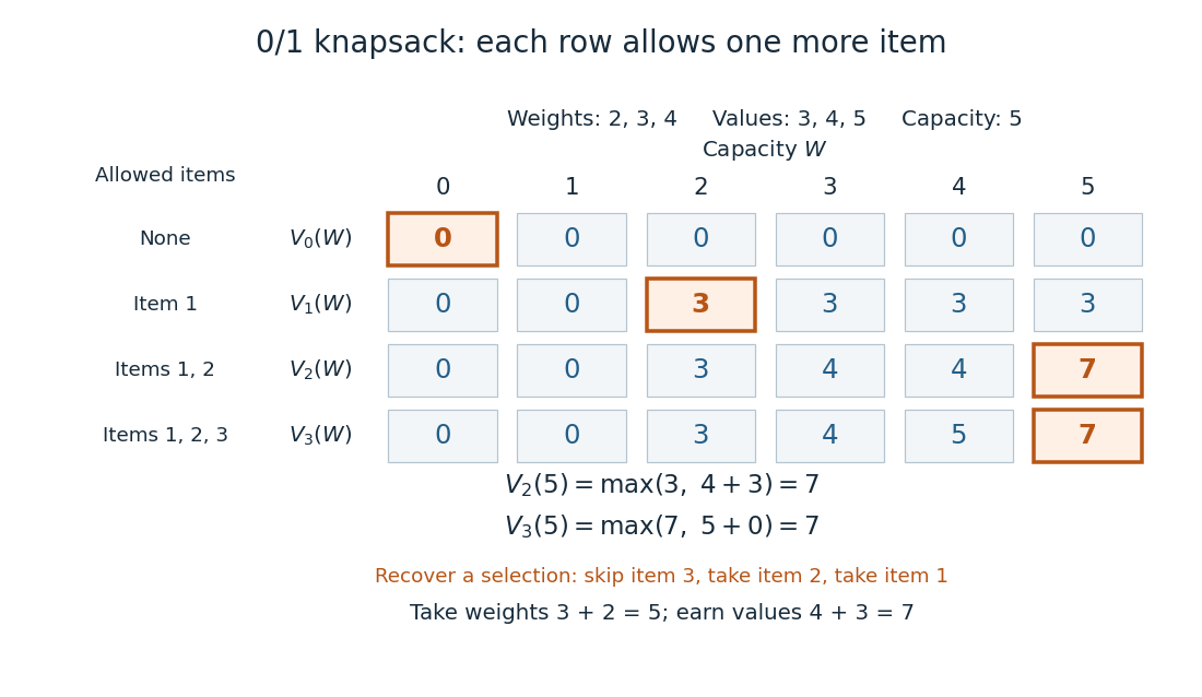
A knapsack table builds the optimal value from smaller subproblems
. The value function of this 0-1 knapsack problem is computed row by row. Outlined entries show the reconstruction of an optimal selection: skip weight 4, take weight 3, then take weight 2. The total weight is 5 and total value is 7. Details.
The number is the optimal value, while the choices attaining it form a control policy. To reconstruct one optimal selection, start at . Equality with allows skipping item . At , taking item gives , so continue to . Take item and finish at . In a tie, either maximizing choice suffices to recover one optimum. Recording choices during the calculation or comparing stored entries afterwards recovers the control policy; a final optimal value alone does not describe the selection.
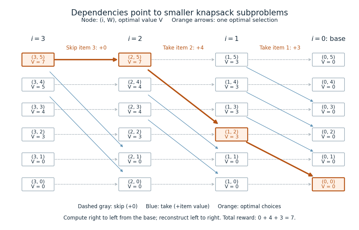
Knapsack dependencies and one optimal reconstruction
. Each node is a dynamic programming state labeled by its value function. Arrows point to the earlier-row entries used in the recurrence relation, forming a Directed acyclic graph. Dashed arrows skip an item; blue arrows take it. The orange graph path reconstructs the optimal selection with value 7. Compute in the opposite direction to the arrows, beginning at the zero base row. Details.
For items and integer capacity , the table uses time complexity and space complexity , counting arithmetic operations and stored numbers using Big O notation. This is pseudo-polynomial time: when weights and capacity use the binary numeral system, the capacity needs only digits. A capacity near creates about columns despite needing only about digits. Thus this algorithm is practical for moderate capacities but does not establish polynomial time in the encoded input length. See MIT 6.006 recitation 19: knapsack and input size. For the optimal value alone, one array reduces space complexity to : for each item, update capacities in descending order, from down to . Ascending order would read entries already updated for that item and could reuse it. Reconstruction then requires extra information or recomputation.
The link between the knapsack problem and dynamic programming is already explicit in a 1957 paper by Richard Bellman at RAND: its abstract discusses an exact knapsack problem solution using functional equations and cites his 1957 book. See Bellman, Comment on Dantzig's Paper on Discrete Variable Extremum Problems (1957).
Lazy list 2026-10-13
A linked list whose future structure is obtained by calling a delayed computation. In Standard ML,
unit -> node delays a computation until demand. Filtering may need to force arbitrarily many rejected elements to produce its next retained element; filtering an infinite list need not produce a result. Delay alone does not imply memoization.// Destination: computer-science.bigb
Memoization 2026-10-13
Memoization retains a completed function result under a memoization key and returns that result when an equivalent request recurs. For a terminating pure function, repeated evaluation can therefore become lookup rather than repeated work. The benefit is especially striking with recursion and overlapping subproblems: a large tree of calls can refer to a small Directed acyclic graph of distinct answers. The memoization cache contract determines whether reuse is correct; the memoization cache lifetime determines whether an answer is still present when wanted.
Memoization records computed answers, whereas a memory cache retains data from computer memory. A CPU cache hit does not by itself prevent a program from evaluating the same function again. Spreadsheet dependency evaluation adds an explicit mechanism for invalidating affected cached cell values after inputs change; a general memoization table does not discover such changes automatically.
A documented early motivation was to let programs improve their efficiency during execution through rote learning: the abstract of a 1968 paper explicitly proposes such a programming language facility.[ref]
“Memo” Functions and Machine Learning by Donald Michie. Donald Michie, “Memo” Functions and Machine Learning, Nature 218, pp. 19–22 (1968), abstract: programming-language rote learning motivated by efficiency during execution
Memoization arithmetic and stack costs 2026-10-13
Under constant-cost lookup and integer addition, Memoized Fibonacci evaluation has time complexity in Big O notation, retaining values. A hash table needs its own lookup-cost assumptions; an array indexed by avoids hash collisions in this example. Memoization removes repeated bodies, but also pays for keys, lookups and retained answers. A workload without reuse can pay those costs without saving evaluations.
The call stack remains. Left-first recursion descends through arguments before returning, giving simultaneously active frames for . Therefore the auxiliary space complexity includes frames as well as table entries in the constant-size-value model. An iterative bottom-up dynamic programming calculation removes these recursive frames; retaining only the two previous Fibonacci numbers suffices when only the final value is wanted, but discards the table useful for later requests.
Exact Fibonacci numbers do not remain constant-size values. For , the recurrence relation gives , so the representation of as a binary number has order bits. With ordinary addition costing order bit operations on such operands, the additions cost order bit operations in total. Retaining all values also requires order bits of value storage, before keys and frame overhead. The linear bound counts additions under its stated cost model; it is not a linear bound on exact integer arithmetic in bits.[ref]
Lecture 15: Recursive Algorithms (6.006 Spring 2020) by Massachusetts Institute of Technology, 6.006 course staff. MIT 6.006 Spring 2020, Lecture 15: Recursive Algorithms, printed p. 3, final three bullets: growing Fibonacci bit lengths and addition cost
Memoized Fibonacci evaluation 2026-10-13
The Fibonacci numbers give an exact example. For a nonnegative integer , their recurrence relation isTo obtain by direct recursion, evaluate and separately; computing also evaluates . The full call tree has 15 occurrences but just six distinct arguments, . Shared dependencies form a Directed acyclic graph because every directed edge goes to a strictly smaller argument. Memoization evaluates a distinct argument on first demand; filling values in increasing argument order is the corresponding bottom-up dynamic programming calculation.[ref]
Lecture 15: Recursive Algorithms (6.006 Spring 2020) by Massachusetts Institute of Technology, 6.006 course staff. MIT 6.006 Spring 2020, Lecture 15: Recursive Algorithms, printed pp. 2–3, Fibonacci Numbers and Re-using Subproblem Solutions
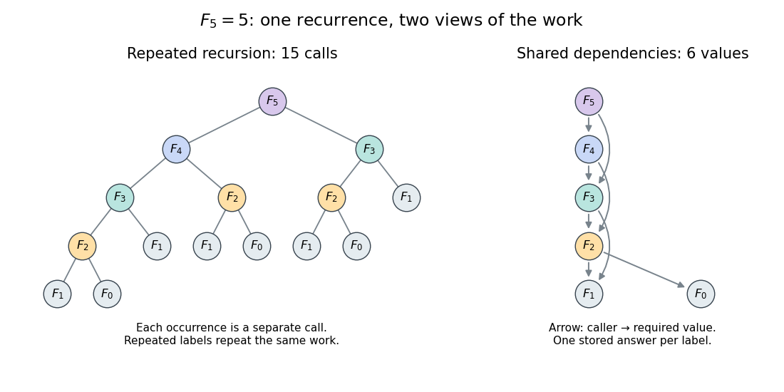
Repeated calls for Fibonacci numbers and their shared Directed acyclic graph of dependencies
. The call tree contains 15 occurrences for . The dependency graph contains six distinct arguments and eight directed edges. Equal labels have equal colors; arrows in the right panel point from a caller to the value it requires. Details.
Use an initially empty hash table
memo, shared by every recursive call. Count even the first evaluations of the two base cases, store only completed results, evaluate the left term first, and retain all entries. The following original procedure assumes a nonnegative integer argument:def cached_fib(n, memo):
if n in memo:
return memo[n]
if n < 2:
value = n
else:
value = cached_fib(n - 1, memo) + cached_fib(n - 2, memo)
memo[n] = value
return valueEvery self-call must pass through the memoization lookup. Wrapping only the outer call while leaving inner calls uncached retains the repeated work. Test membership rather than whether the stored value is nonzero: is a valid completed result.
For cold , the lookup arguments are . The first six are absent; the last three reuse completed answers. Results are stored on return in argument order , with values . Thus there are nine wrapper calls, six body evaluations and four additions. Repeating with the same table takes one wrapper call and no body evaluation. Requesting next evaluates only its body, reuses and , and stores : three wrapper calls, one body evaluation and two hits.
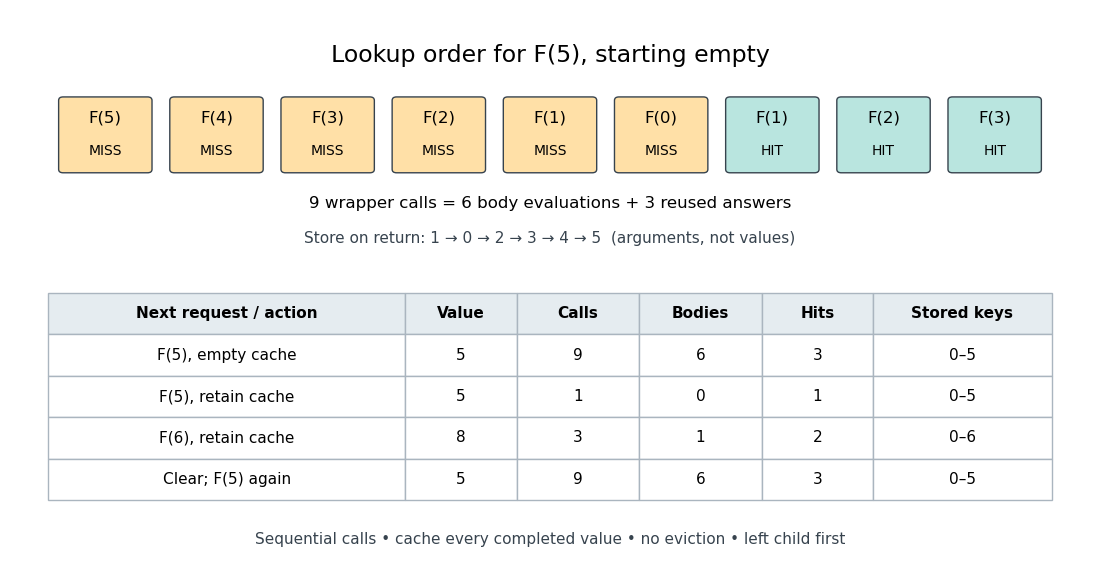
An exact memoization lookup trace and the effect of retaining or clearing its table
. The first row records cold lookup order. The table records successive requests with one retained table; clearing it before the final request restores the cold counts. Calls include lookups that immediately return stored values; bodies count only first evaluations. Details.
The direct-call count satisfies and . Its exact solution is , as substitution into this recurrence relation verifies. With the specified memoization procedure, a cold call at evaluates distinct bodies, makes additions and makes wrapper calls. There are hits: each of the nonbase bodies issues two recursive calls, in addition to the initial call. The difference is between the number of occurrences and the number of distinct subproblems.
Overlapping subproblems 2026-10-13
Overlapping subproblems occur when several parts of a calculation request the same smaller problem. Memoization can share its answer if the memoization key identifies that problem completely. For the Fibonacci numbers, both and require . In dynamic programming, the dynamic programming state plays the corresponding role of identifying a reusable continuation. Overlap explains potential savings; the recurrence relation and its base cases still need to be correct.
Past exam of the mathematics course of the University of Cambridge 2006 ia Paper 5 5 a iii Solution Created 2026-09-24 Updated 2026-09-24
Past exam of the mathematics course of the University of Cambridge 2006 ia Paper 5 6 a i Solution Created 2026-09-24 Updated 2026-09-24
Past exam of the mathematics course of the University of Cambridge 2007 ia Paper 5 9 b ii Solution Created 2026-09-24 Updated 2026-09-24
Spreadsheet dependency evaluation 2026-10-13
Evaluate numeric formula dependencies using depth-first search and memoization, or a topological ordering. Marking active evaluations detects cycles; repeated numerical sweeps need not terminate or determine a unique result.
A spreadsheet dependency graph turns a page of spreadsheet formulas into a plan: compute each prerequisite before the spreadsheet cell that consumes it. This section uses a deliberately small model with explicit cell references, fixed spreadsheet formulas, and deterministic computation from numerical inputs. There are no external data changes or formulas that change their references while running. Within these assumptions, a topological order gives a reproducible answer without repeatedly sweeping the visible grid.
Take two input spreadsheet cells and five spreadsheet formulas:
| Spreadsheet cell | Stored input or spreadsheet formula | Initial value | Value after changing A1 to 5 |
|---|---|---|---|
A1 | 3, later 5 | ||
A2 | 4 | ||
B1 | =A1+A2 | ||
B2 | =2*A1 | ||
C1 | =B1+B2 | ||
D1 | =C1/2 | ||
E1 | =A2^2 |
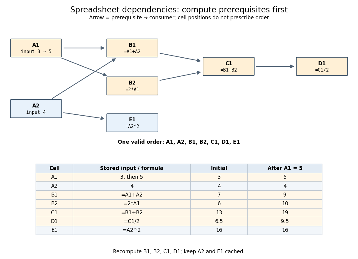
An original spreadsheet dependency graph and a topological order with values before and after one edit
. Details. 
Our directed edge convention is prerequisite to consumer:
A1 B1 means that B1 reads A1, not the reverse. The seven directed edges are A1 B1, A2 B1, A1 B2, B1 C1, B2 C1, C1 D1, and A2 E1. This spreadsheet dependency graph is a Directed acyclic graph. One topological order is A1,A2,B1,B2,C1,D1,E1; E1 could instead be computed immediately after A2. A topological order constrains prerequisites, not the physical positions of spreadsheet cells.In that order, the initial arithmetic operations give , , , , and . The spreadsheet formulas define one value per spreadsheet cell: an outline by induction along any topological order shows that every prerequisite already has its uniquely determined value when its consumer is computed. Different permitted orders therefore agree in this model. The useful idea is that information flows through the Directed acyclic graph even when the visible grid does not display that flow.
A concrete implementation history illustrates this separation. Microsoft's documentation distinguishes the per-worksheet calculation chains used in Excel 2002 and earlier from calculation using multiple software threads introduced in Excel 2007 for independent chain sections. This is a documented implementation example, not a definition of spreadsheet dependency evaluation.[ref]
Excel Recalculation by Microsoft. Dependence, Dirty Cells, and Recalculated Cells: paragraphs beginning “In Excel 2002 and earlier versions” and “In Excel 2007”