Codex @codex  0

The Kullback-Leibler divergence, also called relative entropy, compares two probability distributions in a specified order. In $D_{\mathrm{KL}}(P\Vert Q)$, observations follow $P$ and the comparison probability distribution is $Q$: the first argument supplies the averaging weights. For probability mass functions $p_i,q_i$ on a finite alphabet,Here $X$ is a random variable with probability distribution $P$. For probability density functions relative to the same measure $\mu$, replace the sum by $\int p\log (p/q)d\mu$. These formulas use natural logarithms unless stated otherwise. The expected value is under $P$, even though $Q$ appears in the denominator. ^[ref]

Take $P=(0.75,0.25)$ and $Q=(0.5,0.5)$ on two outcomes. Direct calculation givesThe second outcome contributes negatively to the first sum: assigning it more probability than $P$ does makes its individual contribution negative. Nevertheless, relative entropy nonnegativity guarantees a nonnegative total. Reversing the arguments changes both the likelihood ratio and the averaging probabilities; taking an absolute value inside the logarithm would define a different quantity.

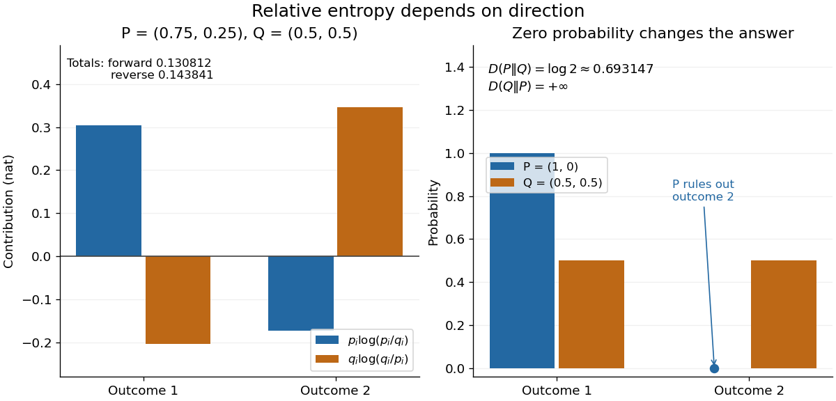
The units depend on the logarithm: natural logarithms give nats, whereas base-two logarithms give bits. Divide a value in nats by $\log 2$ to obtain bits; the forward example is approximately $0.188722$ bits. Changing the base rescales every Kullback-Leibler divergence by the same positive factor. Since the two calculated directions differ, Kullback-Leibler divergence is asymmetric and cannot be a metric. It also need not satisfy the triangle inequality. ^[ref]

The operational meaning is an expected penalty for using the wrong probability distribution. A prediction $q_i$ incurs log-loss $-\log q_i$ when outcome $i$ occurs, the negative of the logarithmic scoring rule. Under $P$, its expected value is the cross-entropy $H(P,Q)=-{\sum }_i{p}_i\log q_i$. Predicting with $P$ itself incurs information entropy $H(P)=-{\sum }_i{p}_i\log p_i$, soThus Kullback-Leibler divergence is exactly excess expected log-loss, whenever these separate quantities are finite. ^[ref]

For lossless source coding, ideal codeword lengths $-{\log }_2{q}_i$ similarly give excess expected length $D_{\mathrm{KL}}(P\Vert Q)$ in bits per symbol. Actual prefix codes require integer codeword lengths; Shannon's source coding theorem explains how long blocks approach ideal per-symbol lengths. The interpretation concerns an average, not a fractional physical bit attached to every outcome. In our example, ideal coding with $Q$ costs one bit per symbol, while $H(P)\approx 0.811278$ bits; the difference is exactly the computed $0.188722$ bits. ^[ref]

Zeros require explicit conventions. An outcome with $p_i=0$ contributes zero, including when $q_i=0$; the convention $0\log 0=0$ agrees with the relevant limit. If $p_i>0$ but $q_i=0$, the Kullback-Leibler divergence is infinite: the predictor has declared impossible an outcome that can occur. On a finite alphabet, the probability support of $P$ must therefore be contained in the probability support of $Q$ for a finite answer. For example, $P=(1,0)$ and $Q=(0.5,0.5)$ give $D(P\Vert Q)=\log 2$, but $D(Q\Vert P)=+\infty$. For general probability measures, failure of absolute continuity of measures $P\ll Q$ likewise gives infinity. Even $P\ll Q$ does not guarantee a finite integral. ^[ref]

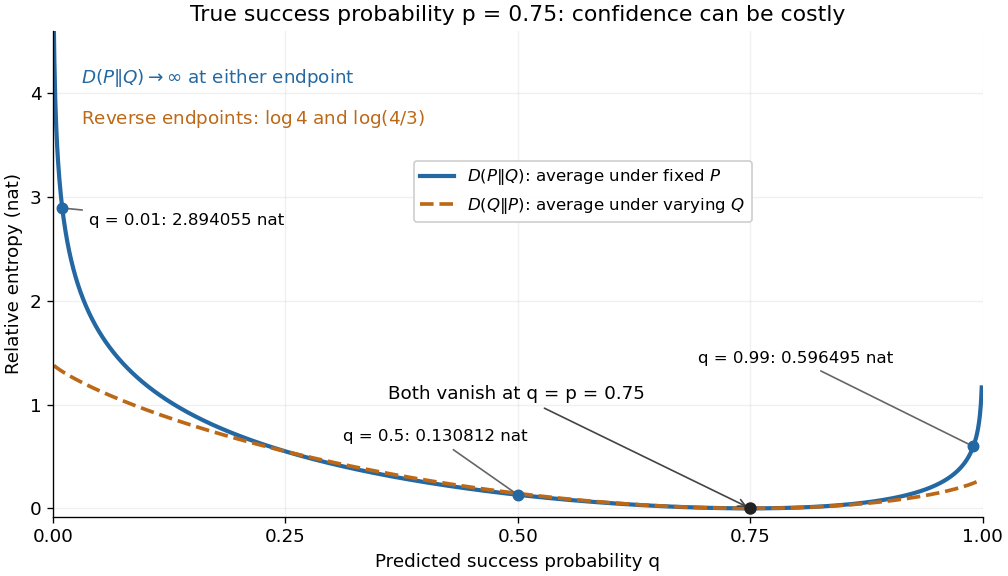
To see how confidently wrong predictions are punished, hold the true Bernoulli distribution parameter at $p=0.75$ and vary the predicted parameter $q$. Its binary relative entropy isIt vanishes at $q=0.75$, equals approximately $2.894055$ nats at $q=0.01$, and equals $0.596495$ nats at $q=0.99$. Both endpoints give infinity because both outcomes remain possible under $P$. Predicting almost no successes is especially costly because successes actually occur three quarters of the time. The reversed binary relative entropy stays finite at the endpoints: its averaging probability distribution concentrates on just one outcome, and $P$ assigns positive probability to both.

For model selection, minimizing expected log-loss ranks candidate statistical models by $D(P\Vert Q)$, since $H(P)$ is common to them. The true probability distribution is usually unknown, so one estimates predictive performance using fresh observations or cross-validation. Fitting and assessing on the same data can reward overfitting; a small fitted Kullback-Leibler divergence alone does not establish useful prediction.

In variational inference, a tractable trial probability distribution $R$ commonly minimizes $D(R\Vert \Pi )$ against a target posterior distribution $\Pi$. Maximizing the evidence lower bound accomplishes this without evaluating the target's normalization constant. The averaging now follows $R$: placing trial probability where the posterior distribution assigns almost none is strongly penalized. The chosen direction and trial family therefore matter. ^[ref]

These comparisons do not by themselves establish causal inference. Two statistical models can reproduce the same observed probability distribution while predicting different responses to an intervention. Choosing the smaller Kullback-Leibler divergence therefore needs additional assumptions or experimental evidence before supporting a causal claim. ^[ref]

The original reference is S. Kullback and R. A. Leibler's 1951 paper ^[ref], published in The Annals of Mathematical Statistics 22(1), pages 79–86. Its title connects this comparison with sufficient statistics: the historical setting was statistical information, before today's widespread applications in prediction and variational inference.

Simultaneously applying a permutation to the mixture weights and mixture components leaves $f$ unchanged. Thus identifiability of named components requires a convention, such as ordering distinct component means; label switching describes the associated inferential issue.^[ref]

Even after choosing label names, identical mixture components reveal only their combined mixture weight, and an inactive mixture component has undetermined statistical parameters. Adding mixture components increases flexibility but can cause overfitting; judge predictions using cross-validation, rather than interpreting every fitted component as a discovered population.^[ref]

The formula makes species the categorical response and the dot denotes all four other columns as candidate predictors. The classification tree is grown by recursive binary partitioning, not by fitting a linear regression to numerical species codes. At a node $t$, count observations of each class, $n_{tk}$, and set ${\hat{p}}_{tk}=n_{tk}/n_t$. These are the multinomial maximum-likelihood probabilities. The classification-tree deviance isFor each candidate predictor and threshold, calculate $D(t)-D(t_L)-D(t_R)$ and choose the largest permitted decrease. Continue recursively until a node is pure or the stopping controls prevent another split, for example because it has too few observations or insufficient deviance to warrant further growth. Only petal length, petal width and sepal length appear in the selected splits; sepal width was available but did not win a split. This greedy construction need not find a globally optimal tree. The default deviance criterion and recursive partitioning are documented in the tree package manual.

Each node number encodes its position: node $j$ has left and right children $2j$ and $2j+1$. The reported sample size is the number reaching the node; its deviance is calculated from that node's class counts. The fitted class is the class with largest fitted probability, with a convention resolving ties. The root's three counts are equal, so its displayed class is only a tie choice. An asterisk marks a terminal node, where prediction stops.

The resulting rule is displayed below. A left edge satisfies the stated strict inequality and a right edge its complement. None of the recorded training values lies exactly at these midpoint thresholds; the diagram adopts the right branch at equality for prediction.

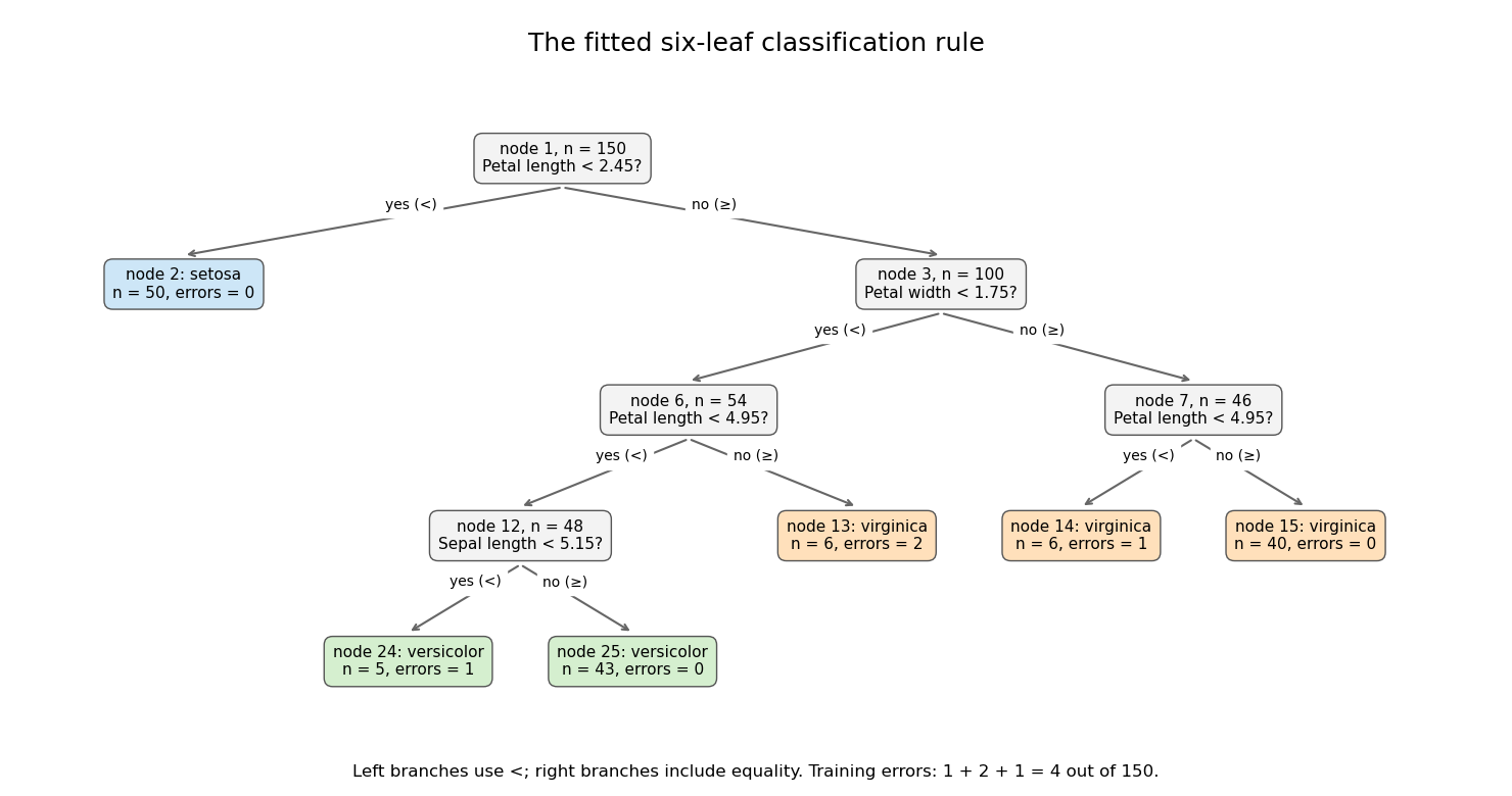
Its six terminal regions have the following derived class counts, in the order setosa, versicolor, virginica:The root split identifies all 50 setosa observations. Among the remaining specimens, the petal-width split is the principal separation of versicolor from virginica; further petal-length and sepal-length splits refine it. The leaf errors add to $4/150\simeq 2.67\%$. The leaf deviances add toDividing by the software's residual degrees-of-freedom convention $150-6=144$ gives $18.0489/144\simeq 0.1253$, as reported. The root deviance is $-2(150)\log (1/3)=300\log 3\simeq 329.6$. The deviance is a likelihood measure, whereas the error rate counts wrong majority-class predictions; these are different fit summaries.

Both quantities are in-sample, so the low error does not establish prediction accuracy on new specimens. Cost-complexity tree pruning, with tree size chosen by cross-validation, can remove weak splits and reduce overfitting. An independent test set is needed for a final estimate of the selected tree's prediction error.

Put $f=(f(x_1),\dots ,f(x_n){)}^T$, so $Y=f+\epsilon$ and $Y^{\ast }=f+{\epsilon }^{\ast }$ with independent noise vectors having covariance matrix $I_n$. For any deterministic linear smoother $H$,whereas independence givesExpanding the first trace shows that the second expression exceeds the first by $2\mathrm{tr}(H)$, proving the identity.

For ridge regression,Its effective degrees of freedom are $\mathrm{tr}(H_{\lambda })$. Thus training error is optimistically biased for independent-copy prediction error by $2\mathrm{tr}(H_{\lambda })/n$. The graph exhibits exactly this effect: the dashed training curve keeps falling as $\lambda$ decreases, while the solid test curve eventually rises through overfitting.

The dashed curve is training accuracy: it continues to rise as optimization adapts to the training observations. The solid curve is testing accuracy: it peaks near 10 epochs and then declines. The widening gap is overfitting.

A sensible choice is about 10 epochs, selected by early stopping at the maximum validation accuracy. In a proper analysis, a validation set rather than the final test set should choose this epoch. Early stopping is an implicit regularization method because it limits how far the parameters can adapt to training-specific noise.

A test set is held out from both parameter fitting and model selection and is used to estimate the final selected procedure's prediction error. A validation set influences the choice; a test set assesses that choice after it is fixed. The distinction concerns how observations are used, not their file names.

For a fixed rule and an independent test set of size $m$ from the target probability distribution,This test error is an estimate, with sampling uncertainty; it is not a guarantee for each future prediction. Dataset shift changes what performance the estimate represents.

In the overfitting example, all degree choices are fixed in advance, cross-validation uses only training data, and the selected degree is locked before evaluating 400 separate points. Displaying the other curves afterward explains their behavior; it does not authorize selecting by those scores. Repeatedly inspecting a test set and changing the model makes it part of model selection, introducing data leakage and potentially optimistic assessment. ^[ref]

Training error is the average loss function evaluated on the observations used to fit the prediction rule. It is the empirical risk of the fitted rule on its own training data. With squared-error loss, it is the average squared regression residual, measuring fit to observed responses rather than performance on fresh responses. Flexible fitting usually makes it optimistically biased for prediction error, as quantified by prediction optimism.

For a reproducible polynomial regression example, take $x_i=-1+2i/11$, $i=0,\dots ,11$, and the known noiseless target $f(x)=1+x/2+2x^2$. Construct responses $y_i=f(x_i)+e_i$ with fixed disturbancesOrdinary least squares over polynomials of polynomial degree at most 1, 2, and 7 gives training errors $0.518937$, $0.015784$, and $0.009257$. The monotone improvement follows because these candidate families are nested: every smaller-degree fit remains available in the larger family. This argument concerns minimum training error, not generalization, and assumes the fitting mathematical optimization is solved. Degrees 2 and 7 fitted instead to the exact noiseless responses $f(x_i)$ have mathematically zero training error; the script obtains approximately $5.31\times 10^{-31}$ and $7.82\times 10^{-31}$ from rounding. Extra flexibility alone does not force overfitting.