Within-model inference. The data are the measurements, specifies a statistical model including its sampling assumptions, and is its unknown parameter or parameter vector. The posterior describes parameter uncertainty after the observation. The likelihood describes how that observed data set depends on a proposed parameter. The parameter prior encodes information before these data. The evidence is the prior predictive probability density of the data and normalizes the posterior:For continuous observations the likelihood and evidence are densities in data space, rather than probabilities of one exact observation. The evidence compares different models only when they use the same data and reference measure.
Uniform parameter priors. Normalize each model's top-hat prior, so inside its allowed interval and zero elsewhere. ThenThus evidence is the average likelihood over the allowed parameter range, not its maximum and not the unnormalized area alone. Interpret the supplied measured distribution as proportional to a common likelihood, , where the common constant cancels in model comparisons. If that distribution were instead a posterior calculated using a nonuniform reference prior, it would first need to be divided by that prior. No such alternative prior is specified here.
Evidence calculation. Put . The three integrals, divided by the same , areConsequently the three pairwise Bayes factors may be given asB has the largest evidence. Model A is narrow but lies away from the likelihood peak. Model C contains that peak but spreads much of its normalized prior over less well-fitting values. Model B concentrates its parameter prior near the peak and achieves the best average. Width is therefore not a universal penalty by itself: changing an interval can also improve its location. At fixed centre near a localized likelihood peak, extending the interval into poorly fitting values dilutes the evidence.
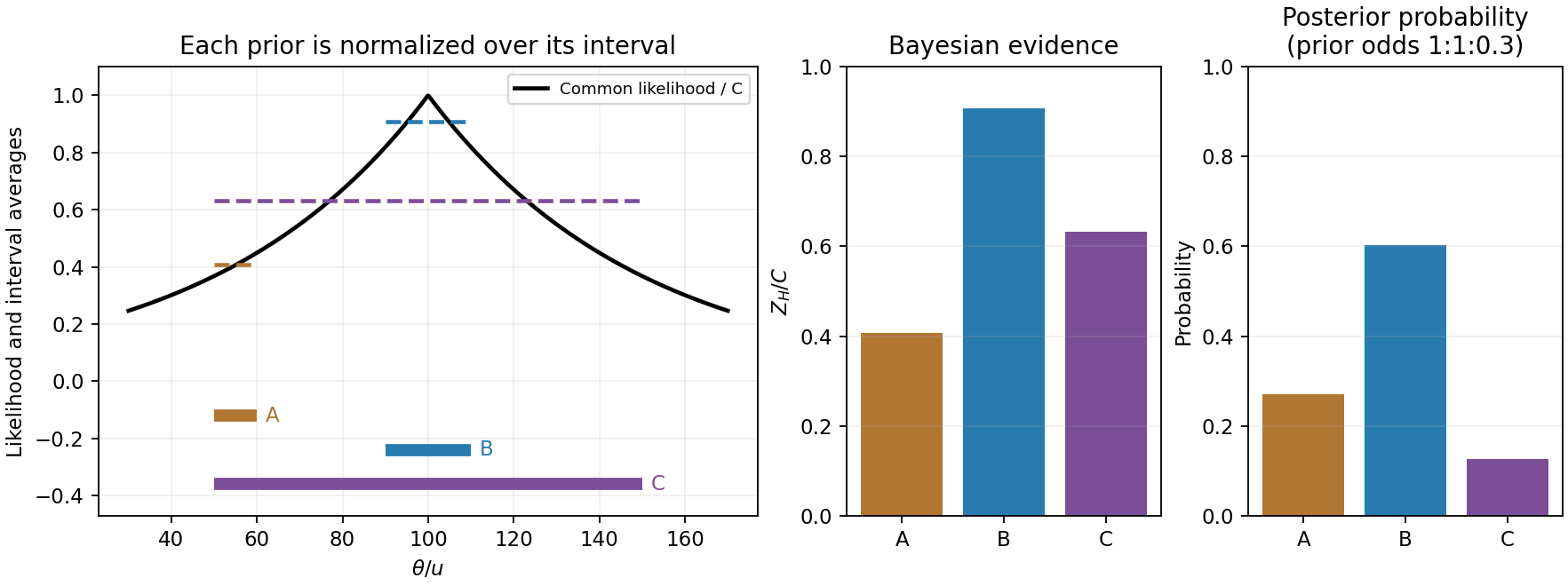
Original likelihood averages over the three top-hat prior intervals; bars show evidence and separately prior-weighted model probabilities
. Details. 
Between-model prior information. The supplied are model prior odds, distinct from each model's uniform parameter prior. They multiply the evidences to give posterior model weights. The corresponding posterior odds areNormalizing these weights gives , and . B is preferred with either equal model priors or the stated theoretical prior odds. Multiplying by changes posterior odds; it does not redefine the Bayes factors.
Euclidean luminosity selection. In a flux-limited catalogue, a source with isotropic luminosity is detected out toA homogeneous Euclidean population with intrinsic luminosity function is sampled approximately as . Brighter objects occupy a much larger accessible volume and are overrepresented; at a fixed large distance the faint tail is missing entirely. This is Malmquist bias. Using the selected population as if it were representative can bias luminosity calibrations or inferred correlations with . A selection function, a volume-limited sample, or appropriate accessible-volume weighting can address the sampling effect, subject to completeness assumptions.
The Euclidean derivation concerns flux-limited luminous objects or selected tracers associated with the structures. A CMB temperature map is a diffuse surface-brightness field on a cosmological last-scattering surface: it is not automatically a Euclidean catalogue of identical inverse-square point sources. For a particular CMB-structure catalogue, its actual detection statistic and selection function must be specified before applying this luminosity-weighting law quantitatively.
Delay-compensated geometry. Choose an east-west baseline vector and let the upward unit vector be . A ray direction at zenith angle in their plane has . Its signed geometric path difference is . Removing the phase-centre delay leaves the residual pathWith the receiver ordering chosen to give positive phase for this path, a complex correlator measuresThe reverse ordering complex-conjugates the expression without changing its information. A single real multiplier supplies its cosine component; the stated exponential represents an in-phase/quadrature correlator. Equal cable lengths to the central correlator remove a fixed instrumental difference but do not remove the changing geometric delay. Pointing the antennas and electronically compensating the path are separate operations.
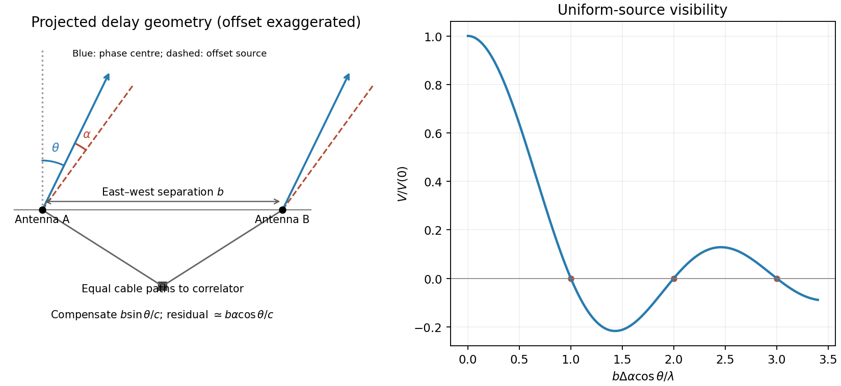
Original east-west interferometer geometry and normalized visibility of a centred one-dimensional uniform source
. Details. 
Resolved uniform source. Contributions from mutually incoherent sky elements add as brightness-weighted complex visibilities. Put over and zero elsewhere, and define . Integrating givesThereforeThe zero-argument value is defined by continuity as one. Normalization by isolates the visibility shape from total flux. The first null occurs when the source spans one fringe period, . A negative real visibility beyond a null is a phase reversal, not negative surface brightness.
Path-compensation precision. A finite observing band sets a coherence envelope. For a rectangular band of width , an uncorrected residual delay multiplies the correlation byCoarse delay steps must leave if decorrelation is to be small. Thus a coarse path-step scale must be well below the coherence length , with the precise bound determined by the tolerated amplitude loss and maximum quantization residual. A digital fine-delay or phase-rotation system can separately correct the central-frequency phase.
If there is no such carrier-phase correction, the steps must also be a small fraction of to avoid large untracked phase jumps or time-averaging loss. For a step rounded to the nearest setting, and the maximum carrier-phase error is . Bandwidth controls coarse group-delay decorrelation; wavelength controls the precision of untracked carrier phase. No numerical delay step can be inferred from the central frequency alone without a bandwidth, loss tolerance and compensation architecture. Earth rotation additionally sets how rapidly the delay setting must be updated.
Largest sampled angular scale. For a near-zenith view take the shortest projected baseline as . At , . The inverse shortest spatial frequency givesThis is an order-of-magnitude largest fringe scale. A convention defining maximum recoverable source size as would instead give about arcminutes; source profile, weighting and projected baseline coverage determine the operational value. The antenna diameter and primary beam can further restrict the usable field but were explicitly neglected in the source's initial idealization. Ten antennas supply pairwise baselines; their number improves sampling and sensitivity, not the inverse-shortest-baseline scale by a factor of ten. The longest baseline is not supplied, so the finest synthesized resolution is not numerically fixed.
A suitable observing programme. A compact centimetre-wave array is well suited to CMB temperature anisotropy on degree to sub-degree scales sampled by its baselines, and, with sufficiently long baselines and suitable foreground control, thermal Sunyaev-Zeldovich structure in galaxy clusters. At the thermal Sunyaev-Zeldovich signal is a decrement relative to the CMB. The compact baselines retain sensitivity to extended brightness features; the spatial frequencies measured by each baseline have a direct statistical interpretation in CMB analysis.
Compared with lower radio frequencies, synchrotron foregrounds are generally reduced, while thermal dust rises toward higher frequencies; observing near this centimetre-wave atmospheric window is therefore useful, although foregrounds are not absent. Correlation and phase switching reject mean uncorrelated receiver offsets and some instrumental drifts. Receiver thermal noise still contributes variance, and atmosphere, ground pickup or cross-talk can be correlated and require control. Additional long baselines can identify compact radio-source contaminants for subtraction, but the question does not specify enough array geometry to guarantee that capability. There is no zero baseline in ordinary pairwise cross-correlation, so the array does not directly measure the sky monopole or arbitrary larger-scale smooth emission.
Stellar reflex motion. A planet and its host orbit their common barycentre. The star's line-of-sight velocity shifts its absorption lines by at low speeds. A time series can be fitted withHere is true anomaly, the argument of periastron and an arbitrary systemic velocity offset. At small companion mass and known stellar mass, the orbit supplies , not the true planet mass without an inclination constraint. Long monitoring helps distinguish a reproducible Keplerian signal from stellar oscillations, magnetic activity, spots and instrumental trends.
The Lick reference-cell implementation. Starlight passes through a temperature-controlled cell of molecular iodine before entering the Hamilton high-resolution echelle spectrograph. The cell imprints a dense pattern of reference absorption lines on the stellar spectrum, predominantly in the approximately – interval. These lines share the same exposure and downstream optical path as the stellar light. A calibrated high-resolution Fourier-transform iodine spectrum and an iodine-free stellar template allow the wavelength solution and instrumental line-spread function to be fitted along with the stellar Doppler shift. The method corrects shifts and line-shape changes that a separate calibration exposure would not necessarily follow.[ref]
Precision Radial Velocities with an Iodine Absorption Cell by Geoffrey W. Marcy and R. Paul Butler. Marcy and Butler (1992), sections 3–4, printed pages 271–274: Hamilton setup, iodine wavelength interval, templates and in-situ instrumental profile
A useful forward model for one short spectral segment isfollowed by pixel integration, continuum scaling and a fitted wavelength calibration. Here is the intrinsic stellar spectrum, the cell transmission and the instrumental line-spread function. The spectra multiply before convolution; simply dividing a recorded blended spectrum by the laboratory iodine spectrum is not equivalent to this model. The iodine pattern is stationary in the observatory frame while stellar lines move relative to it. Separate spectral segments accommodate wavelength dependence of the instrumental profile.
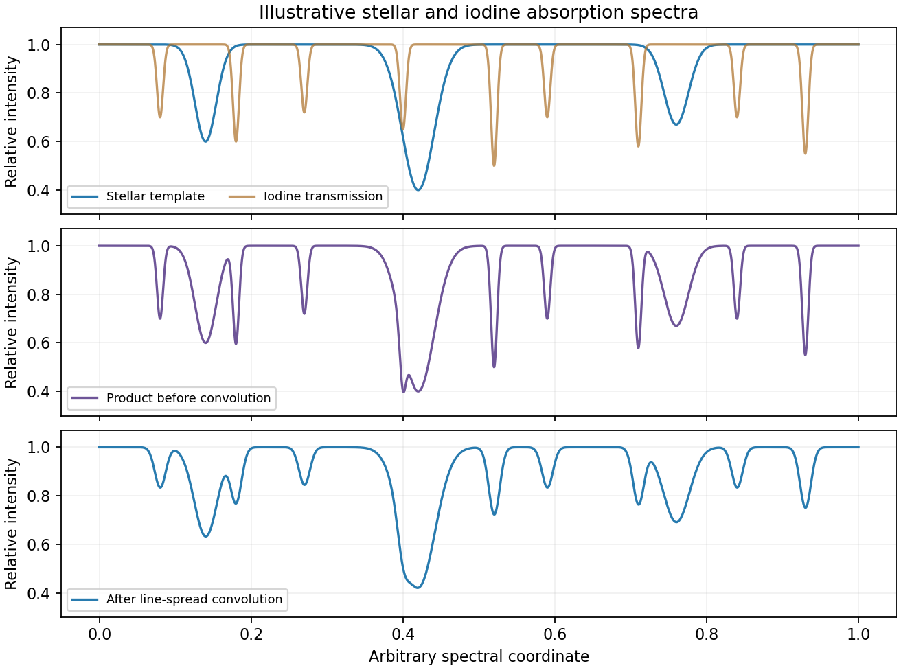
Original synthetic iodine-cell forward model showing multiplication before instrumental convolution; all line positions and strengths are illustrative
. Details. 
Earth's rotational and orbital velocities must then be removed with a barycentric correction using accurate timing, ideally weighted by photon arrival rate. Many stellar lines constrain a shift smaller than one instrumental resolution element; spectral resolution alone is not the velocity error. Photon statistics, template quality, instrumental-profile modelling and intrinsic stellar variability limit the precision. The method measures changes relative to a template and does not by itself provide a perfectly absolute centre-of-mass velocity. No particular discovery, modern precision floor or historical observing performance is assumed here.
Atmospheric turbulence produces time-dependent refractive-index fluctuations and phase errors across the telescope pupil. A large aperture's long-exposure point spread function is broadened approximately to , where is the Fried parameter, rather than the diffraction scale . For fixed turbulence, , so the seeing angle improves weakly as . The atmospheric coherence time scales with divided by an effective wind speed. This temporal scale concerns changing turbulence, not the optical bandwidth's coherence time.
Reduce the disturbance. A good high-altitude site, favourable weather, observing near the zenith, thermal control and dome ventilation reduce atmospheric and local seeing. They improve the uncorrected image but do not remove all high-order wavefront distortion. Active optics slowly maintains the main mirror's figure and alignment; it is distinct from the rapid adaptive correction of atmospheric phase errors.
Correct the wavefront. Adaptive optics uses a nearby natural guide star or artificial laser guide star, a wavefront sensor, a real-time controller and a deformable mirror. A Shack-Hartmann sensor estimates local wavefront slopes; mirror actuators apply the opposite optical-path distortion fast enough to track the atmosphere. A separate fast steering element or the mirror can correct image motion. In an ideal well-corrected direction this approaches diffraction-limited resolution and increases the concentration of light in the central image.
Finite guide-star flux, actuator sampling, control latency and anisoplanatism leave residual errors. A laser beacon samples a finite-height cone rather than the full distant-source cylinder, and a conventional laser reference does not determine absolute tip-tilt, so a natural reference remains useful. Multiple guide stars and multiple conjugate mirrors can widen the corrected field, with extra sensing and reconstruction complexity. These are fundamental geometry and control limits, not claims of a universal corrected sky fraction.[ref]
Adaptive Optics by European Southern Observatory. Single Conjugate Adaptive Optics and Multi-Conjugate Adaptive Optics sections: bandwidth, fitting, anisoplanatism, laser-beacon tilt and cone limitations
Freeze and reconstruct. Short exposures can freeze the instantaneous speckle pattern. Speckle interferometry uses calibrated Fourier statistics to recover diffraction-scale structure; power-spectrum information alone loses phase, while bispectrum or other phase-sensitive measurements support image reconstruction. Lucky imaging selects sharp short frames, registers them and combines them, trading photon efficiency for improved image quality. Tip-tilt alignment alone removes image motion rather than all high-order aberration. These methods require sufficiently bright sources or references and can incur substantial read-noise penalties. Deconvolving a long-exposure image is useful only where a known point spread function and adequate signal preserve information; it cannot recover arbitrarily lost spatial frequencies. Moving to space avoids atmospheric seeing, although it changes the observing platform and its limitations rather than correcting a ground-based telescope.
Weak transitions in dilute gas. A forbidden emission line is a transition absent in the electric-dipole approximation because of its selection rules, but permitted through weaker channels such as magnetic-dipole or electric-quadrupole radiation, sometimes aided by state mixing. It is not an impossible transition. Its upper atomic level is relatively long lived, so collisions can deactivate it before a photon is emitted in dense gas. Low-density astrophysical plasmas allow radiative decay to compete successfully.
In a schematic two-level statistical equilibrium,The critical density is for this simple level system; multiple radiative and collisional channels require summed rates. At each collisional excitation is likely to produce radiation, so . At high density collisional de-excitation suppresses the line relative to this low-density expectation. The rate need not decrease absolutely with increasing density; the suppression is relative to the naive excitation scaling.
A temperature-sensitive ratio. For a Maxwell-Boltzmann electron distribution,where is an effective collision strength. Lines from upper levels with different excitation energies therefore have a strongly temperature-dependent ratio. Using one ion reduces sensitivity to abundance and ionization fraction compared with comparing unrelated species.
A standard example is doubly ionized oxygen: the and angstrom lines descend from toward the ground term, while the angstrom line connects to . The higher excitation threshold makes the auroral line relatively stronger in hotter gas. In the low-density Maxwellian approximation, with slowly varying collision strengths,The numerical form is a useful approximation, not a universal exact atomic law; a multilevel atomic calculation with current collision strengths is needed for precise work.[ref]
Resolving the electron temperature discrepancies in H II regions and planetary nebulae: kappa-distributed electrons by David C. Nicholls and others. Section 4, equation 18 and the following approximation warning; arXiv:1204.3880v2, PDF pages 5–6
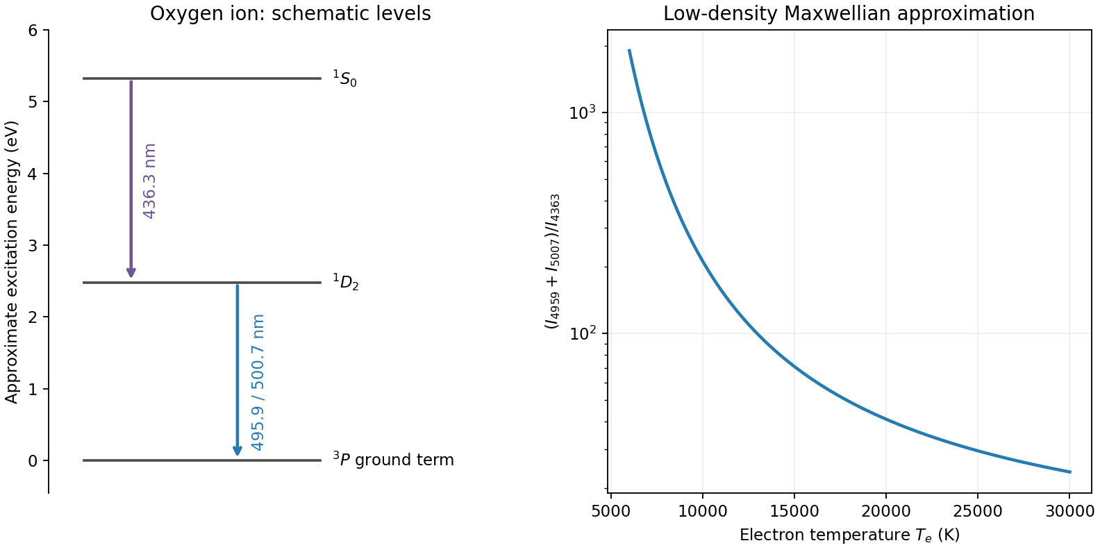
Original oxygen forbidden-line level schematic and low-density Maxwellian temperature-ratio curve; level spacings are approximate
. Details. 
In an active galactic nucleus these lines commonly diagnose the relatively dilute narrow-line gas; dense broad-line gas can collisionally quench them. Measure and deblend the fluxes, subtract continuum and stellar features, correct differential extinction, and check density independently. The ratio mainly tests radiative branching and calibration because both lines share one upper level; it is not the required temperature thermometer. Temperature gradients, multiple density components, shocks, ionization structure and departures from the Maxwellian electron distribution can bias a single inferred temperature. Without a measured ratio and density regime, no particular AGN temperature is numerically determined here.
Measure counts in electrons so that photon and detector noise can be combined directly. For source electrons , aperture pixels, total time , sky rate per pixel, dark-current rate per pixel, reads with rms read noise per pixel, and an independently estimated mean background per pixel of variance , an ideal aperture-sum budget isThe last term represents the propagated calibration uncertainty if it can be treated as a random variance; systematic residuals can instead bias the measurement and need an explicit error model. For a background estimated from independent, equally exposed sky pixels, one approximation is . Correlated resampling, detector cross-talk or a spatially structured sky invalidates the independent-pixel simplification.
Photon counting and sky. Source photon shot noise has variance and cannot be calibrated away. Longer integration or greater throughput improves its fractional error as . Sky photons, including moonlight, airglow and scattered light, add their own Poisson fluctuations. A dark site, appropriate observing time and filter, good baffling and a smaller or optimally weighted source aperture reduce sky contributions. Better seeing or adaptive optics can concentrate a point source into fewer noise-bearing pixels. Sky subtraction removes the mean background but not the random sky photons already recorded, and the sky estimate adds uncertainty of its own.
Dark and read noise. Thermal dark current contributes a mean and shot noise. Cooling reduces its rate; well-matched dark frames remove a reproducible mean and map hot pixels, but do not undo the science exposure's random dark-current fluctuations. Each read adds electronic noise. At fixed total integration, many short exposures add more read variance than fewer long exposures, so use exposures long enough to become sky limited when saturation, cosmic rays and temporal changes permit. Multiple non-destructive reads can help on detectors that support them. Subtracting a bias frame corrects an electronic offset, not the stochastic read noise.
Calibration and non-Poisson effects. Pixel sensitivity differences, illumination gradients, fringes, nonlinearity, imperfect charge transfer and electronic pattern noise leave calibration errors. High-count flat fields, stable operating conditions, linearity calibration, dithering and appropriate detector models help, while the finite signal-to-noise of calibration frames propagates into the result. Cosmic-ray hits, hot pixels, satellite trails and scattered-light artefacts are not ordinary stationary Gaussian noise: identify or mask them, often using several exposures. Overaggressive clipping can remove real transient or compact-source signal.
Atmospheric scintillation adds correlated intensity fluctuations, especially in short bright-star measurements; seeing changes and guiding errors move flux between pixels or apertures. Differential photometry using appropriate reference stars and stable apertures reduces common variations but does not guarantee removal of chromatic or position-dependent effects. For a constant flux-limited source in independent stationary noise the final signal-to-noise usually grows as once background limited; a systematic floor or correlated sky can stop that improvement. Distinguish improvement of calibration, which removes reproducible bias, from elimination of intrinsically random photon arrivals, which is impossible.
Articles by others on the same topic
There are currently no matching articles.