Past exam of the mathematics course of the University of Cambridge / 2005 / iii / Paper 76 (Dynamo Theory)

Use the resistive induction equation with constant magnetic diffusivity,Seek ${\mathbf{B}}_{\mathrm{tot}}=B_0{\mathbf{e}}_z+B(s,z,t){\mathbf{e}}_{\varphi }$. The axisymmetric velocity $\mathbf{u}=s\omega (s,z){\mathbf{e}}_{\varphi }$ is incompressible, and the proposed field is solenoidal. The toroidal magnetic field is parallel to the velocity, so it does not contribute to their cross product. The remaining term isThe uniform axial field has zero vector Laplacian. For the azimuthal part, differentiation of the cylindrical basis gives ${\partial }_{\varphi }^2{\mathbf{e}}_{\varphi }=-{\mathbf{e}}_{\varphi }$. ConsequentlyThere is no source for a radial or axial perturbation, so zero initial values of those components remain zero. Equating the toroidal components provesThe last Laplacian is the scalar axisymmetric Laplacian. The additional $-B/s^2$ term is essential for a vector component in a rotating basis. The source is the Omega effect: rotation that varies along an axial field line winds it into a toroidal magnetic field.

With $s=r\sin \theta$ and $z=r\cos \theta$, radial differential rotation gives ${\partial }_z\omega =\cos \theta {\omega }^{\prime }(r)$. Thus the source is $B_{0}r{\omega }^{\prime }(r)\sin \theta \cos \theta$. Put $B=f(r)g(\theta )$ with $g=\sin \theta \cos \theta$. The toroidal diffusion operator isDirect differentiation of $g$ makes the bracket $-6g$. Therefore the steady radial equation isDefine $I(r)={\int }_0^r{x}^4\omega (x)dx$ and $h=I/r^3$. Since $I^{\prime }=r^4\omega$,so $h^{\prime \prime }+2h^{\prime }/r-6h/r^2=r{\omega }^{\prime }$. Taking $f=-B_{0}h/\eta$ proves the steady toroidal induction by spherical differential rotation:Near zero, $I(r)=\omega (0)r^5/5+O(r^6)$, hence $B=O(r^2)\sin \theta \cos \theta$ and is regular. Its leading vector field is proportional to $z(-y,x,0)$, so the apparent azimuthal-basis singularity on the axis is harmless. The rapid decay of $\omega$ makes $I_{\infty }={\int }_0^{\infty }{x}^4\omega (x)dx$ finite, giving $B\sim -(B_0{I}_{\infty }/\eta )r^{-3}\sin \theta \cos \theta$ at large radius. The homogeneous radial solutions are $r^2$ and $r^{-3}$; regularity at zero excludes the latter, and decay at infinity excludes the former. Thus these boundary requirements also single out the displayed solution in this angular sector.

Let $\ell$ be the characteristic radius over which the differential rotation changes, with angular velocity of order $\Omega$. The winding source has magnitude $F\sim B_0\Omega$. For times too short for appreciable magnetic diffusion, the zero initial toroidal magnetic field therefore grows as $B\sim B_0\Omega t$. In the steady balance, $F$ is opposed by $\eta B/{\ell }^2$, giving $B_{\mathrm{steady}}\sim B_0\Omega {\ell }^2/\eta$. Comparing these amplitudes gives the diffusive establishment time of a wound toroidal field:With $R_m=\Omega {\ell }^2/\eta$, this is $R_m$ rotation times and the steady toroidal amplitude is of order $R_m{B}_0$. Thus high electrical conductivity makes establishment very slow even though winding begins immediately.

More precisely, if $\mathcal{L}={\nabla }^2-s^{-2}$ on regular toroidal magnetic fields, the solution with zero initial value satisfies $B(t)=B_{\mathrm{steady}}-e^{\eta t\mathcal{L}}{B}_{\mathrm{steady}}$. The residual relaxes diffusively. In the unbounded domain, ${\ell }^2/\eta$ estimates equilibration of the rotating region; exact establishment at every radius is only an asymptotic statement, with diffusion on scale $r$ taking order $r^2/\eta$. As $\eta \to 0$, the time diverges and the prescribed-flow ideal solution continues its secular winding. In a real fluid, magnetic tension and Lorentz force feedback can modify the differential rotation before the very large kinematic steady amplitude is attained.

A field in a circulation plane has components crossing circular streamlines. Magnetic flux freezing carries those lines with fluid elements at different angular speeds: the lines become spirals, their azimuthal components are stretched, and neighboring turns acquire increasingly small separations. This is a nonaxisymmetric winding and phase-mixing problem.

For illustration, in the ideal limit take the initial horizontal field along $x$ and fix a horizontal plane. With $\chi =\varphi -\omega (s,z)t$, the induction equations giveThe first term describes advection around a circle; the term proportional to $t{\partial }_s\omega$ is the stretching by differential rotation. Spatial variation of $\omega$ also produces phase gradients proportional to $t\nabla \omega$. A rigidly rotating region merely turns the horizontal field, whereas a shearing region progressively winds it up.

Even small magnetic diffusivity becomes important once these gradients are large. Locally a phase mode of azimuthal order $m$ has damping rate of order $\eta m^2|\nabla \omega {|}^2{t}^2$, leading to attenuation of order $\exp [-\eta m^2|\nabla \omega {|}^2{t}^3/3]$. The associated magnetic phase mixing under differential rotation time isFor a horizontal uniform seed, $m=1$; if $|\nabla \omega |\sim \Omega /\ell$, this is ${\Omega }^{-1}{R}_m^{1/3}$, much shorter than the ordinary diffusion time at large $R_m$. Resistive smoothing cancels the closely spaced oppositely directed field and, in persistent circulation regions with an imposed surrounding field, drives flux expulsion from the interiors toward their boundaries. The detailed final distribution depends on the geometry and boundary forcing. Winding alone does not supply a self-sustaining poloidal–toroidal regeneration loop, and magnetic feedback can again limit the kinematic process.

In mean-field electrodynamics, use Reynolds averaging to write ${\mathbf{U}}_{\mathrm{tot}}=\overline{\mathbf{U}}+\mathbf{u}$ and ${\mathbf{B}}_{\mathrm{tot}}=\overline{\mathbf{B}}+\mathbf{b}$, with zero-mean fluctuations. Assume the averaging operation commutes with the derivatives and that resolved quantities vary little across an averaging region. Averaging the induction equation then givesThis is the mean-field electromotive force, a vector correlation with units of velocity times magnetic field. The closure problem is to express this correlation in terms of the resolved field.

In the kinematic regime the flow statistics are prescribed, so the response is linear in the mean magnetic field, after independently excited fluctuation transients have decayed. If the mean-field scale $L$ is much greater than the turbulent scale $\ell$, and its evolution is slow compared with the response memory, expand that response in the local mean magnetic field and its gradients:Without scale separation one generally has a spatially nonlocal and temporally retarded response rather than constant local coefficients.

For homogeneous turbulence the coefficients are independent of position. Invariance under proper rotations makes the rank-two response proportional to ${\delta }_{ij}$, and the isotropic rank-three gradient response proportional to the alternating tensor. Choosing the diffusivity sign convention givesThe alpha effect can regenerate a mean magnetic field, while $\beta$ supplies turbulent magnetic diffusivity. For constant positive $\beta$, $\nabla \times (-\beta \nabla \times \overline{\mathbf{B}})=\beta {\nabla }^2\overline{\mathbf{B}}$ because the magnetic field is solenoidal. Thus the total diffusivity is $\eta +\beta$.

The electromotive vector is a polar vector, whereas the magnetic field is an axial vector. Therefore $\alpha$ is a pseudoscalar and changes sign under reflection; $\beta$ is an ordinary scalar. A nonzero isotropic alpha effect requires broken reflection symmetry, such as nonzero kinetic helicity. If “isotropic” includes reflection symmetry as well as rotations, $\alpha$ must vanish. The dimensions are $[\alpha ]=L/T$ and $[\beta ]=L^2/T$.

Take zero mean flow locally and incompressible fluctuations. Subtracting the averaged induction equation givesThe first-order smoothing approximation omits the second term on the right when solving for $\mathbf{b}$, but retains $⟨\mathbf{u}\times \mathbf{b}⟩$ in the mean equation. For a locally uniform, slowly changing mean magnetic field the forcing becomes $(\overline{\mathbf{B}}\cdot \nabla )\mathbf{u}$.

There are two controlled ways to make the omitted fluctuation term small. At small eddy magnetic Reynolds number $R_m=u_{\mathrm{rms}}\ell /\eta$, diffusion gives $b/B\sim R_m$, so the omitted $ub/\ell$ is smaller than the retained $uB/\ell$ by $R_m$. Alternatively, if $u_{\mathrm{rms}}\tau /\ell \ll 1$ for the fluctuation response time $\tau$, then $b/B\sim u_{\mathrm{rms}}\tau /\ell$ and the short-memory response is perturbative. Mean-field scale separation is additionally required. Merely calling the turbulence weak or assuming that the mean magnetic field is small does not justify the omission.

With homogeneous initial transients removed, the causal linear solution isInsert this into the electromotive correlation. Isotropy gives ${\alpha }_{ij}=\alpha {\delta }_{ij}$, so taking the trace yields the helicity formula for isotropic first-order smoothing:Using the alternating-tensor sign givesThe minus sign follows from ${ϵ}_{imn}=-{ϵ}_{min}$. This derivation specifies the diffusion and correlation weighting, rather than asserting that alpha is proportional to instantaneous helicity for arbitrary turbulence.

If $\eta \tau /{\ell }^2\ll 1$, diffusion over a correlation time is negligible. Define the helicity correlation time byFor an ordinary decaying correlation with nonzero mean kinetic helicity, this gives the familiar estimateIt is the kinetic helicity, not magnetic helicity. Opposite flow handedness reverses the alpha effect. The time-integral formula remains meaningful if the equal-time helicity vanishes or its correlation changes sign, when replacing it by a single positive correlation time may fail. In the same weak-diffusion short-memory approximation the gradient forcing $-(\mathbf{u}\cdot \nabla )\overline{\mathbf{B}}$ gives $\beta =\frac{1}{3}{\int }_0^{\infty }⟨\mathbf{u}(t)\cdot \mathbf{u}(t-\tau )⟩d\tau \simeq {\tau }_U{u}_{\mathrm{rms}}^2/3$; the two correlation times need not be equal.

In the small-$R_m$, slowly varying quasistatic regime, diffusion is instead essential. The response givesFor velocity concentrated at wavenumber $k_0$, this becomes $\alpha =-⟨\mathbf{u}\cdot \mathbf{\varpi }⟩/(3\eta k_0^2)$. Its effective memory is the magnetic diffusion time on the eddy scale. The controlled low-$R_m$ setting is developed in Moffatt's analysis of turbulent dynamo action; the causal-response calculation above also covers short-memory turbulence without assuming that diffusion is always negligible.

For constant isotropic $\alpha ,\beta$ and zero mean flow, the mean induction equation isLet $\overline{\mathbf{B}}=\hat{\mathbf{B}}{e}^{\sigma t+i\mathbf{k}\cdot \mathbf{x}}$, with $\mathbf{k}\cdot \hat{\mathbf{B}}=0$. On this two-dimensional transverse space, $i\mathbf{k}\times$ has eigenvalues $\pm k$. For example, if $\mathbf{k}=k{\mathbf{e}}_z$, the vectors ${\mathbf{e}}_x\pm i{\mathbf{e}}_y$ have these curl eigenvalues. The homogeneous alpha-squared dynamo growth criterion follows fromChoose the circular polarization of the mode to match the sign of $\alpha$. This is an alpha-squared dynamo: the alpha effect supplies both parts of the regeneration loop without differential rotation.

If arbitrarily long wavelengths are permitted, every nonzero alpha has a growing band $0<k<|\alpha |/{\eta }_T$. Maximizing the quadratic givesprovided $k_{\ast }\ell \ll 1$ so the mean-field approximation is valid. A uniform field has $k=0$, zero curl and zero growth; a constant alpha cannot amplify that uniform mode. In a periodic domain of size $L$, the lowest nonzero wavenumber is $2\pi /L$, giving $|\alpha |L/{\eta }_T>2\pi$. Other boundaries and geometries give different critical constants, but the general scale criterion is $|\alpha |L/{\eta }_T$ sufficiently large. Nonzero kinetic helicity alone is therefore not a sufficient finite-domain dynamo criterion: its induced alpha must overcome diffusion on an available mean-field scale.

The geodynamo operates in the electrically conducting liquid of Earth's outer core. buoyancy from thermal and compositional convection supplies motion, while the Coriolis force organizes rotating flow. Rotation together with radial stratification permits kinetic helicity, typically with opposite signs in the two hemispheres. In mean-field language this allows an alpha effect that converts poloidal and toroidal components into one another. A large-scale alpha-squared dynamo is therefore a plausible regeneration mechanism even without dominant differential rotation.

The growth condition compares this regeneration with the sum of molecular and turbulent magnetic diffusion on the core scale. A spherical model must impose the appropriate magnetic matching at the core boundaries and permit spatially varying, generally anisotropic alpha and diffusivity tensors. Rotation selects an axis, and stratification and boundaries select positions, so homogeneous isotropic turbulence is only a local idealization. Such a model can favor a predominantly axial dipole, but the preferred parity and threshold must be found from its global eigenproblem rather than deduced from the plane-wave formula alone. If mean shear is significant, alpha–Omega regeneration can also contribute.

The first-order-smoothing helicity formula is a useful guide to the sign and magnitude of alpha, not an automatically controlled numerical closure for the core. The important convective motions need not have small eddy magnetic Reynolds number or short enough correlation time; scale separation can also be limited. Furthermore, the Lorentz force modifies the flow and its correlations once the field grows. Saturation therefore requires nonlinear feedback, including dynamo quenching and magnetic-helicity constraints where relevant.

The observed field varies and occasionally reverses. A constant-coefficient growing kinematic eigenmode does not itself explain these reversals or select a saturated amplitude. Spatial and temporal variations, competing modes, and nonlinear flow–field interactions must be included. mean-field dynamo theory supplies a physical regeneration mechanism and a testable threshold, while the geodynamo requires a rotating, bounded, nonlinear realization of that mechanism.

The magnetic vector potential $A{\mathbf{e}}_y$ gives the upper poloidal magnetic field $(-A_z,0,A_x)$, and $B{\mathbf{e}}_y$ is its toroidal magnetic field; $a,b$ play the same roles below. This representation automatically satisfies $\nabla \cdot \mathbf{B}=0$. Diffusion acts in both regions. Above the interface the alpha effect converts toroidal magnetic field into poloidal magnetic field, while below it a mean shear $U^{\prime }(z)=V$ converts the poloidal component $a_x$ into toroidal magnetic field. Separating these source regions still allows an alpha-Omega dynamo through diffusion across the interface.

For electromagnetic matching, keep the closure actually represented by these equations. Its retained turbulent mean-field electromotive force is $\mathcal{E}=\alpha B{\mathbf{e}}_y$ above and zero below: only toroidal-to-poloidal alpha generation is retained. Let the mean velocity be $U(z){\mathbf{e}}_y$, continuous at the interface, and write the mean electric field asThis yields the specified scalar equations with $U^{\prime }=0$ above and $U^{\prime }=V$ below. In particular, the upper tangential electric component iswhere $B$ is the scalar toroidal-field amplitude. The other tangential component is $E_y=-\alpha B-\eta {\nabla }^{2}A=-{\partial }_{t}A$.

Assume equal permeability, no imposed singular surface current and ordinary electromagnetic matching. Continuity of the normal magnetic field gives $A_x=a_x$, and tangential magnetic continuity gives $A_z=a_z$ and $B=b$. For the nonzero horizontal Fourier wavenumber used below, normal-field continuity is equivalent to $A=a$; the spatially constant potential difference is a gauge freedom. Continuity of $E_x$, with continuous $U$ and $A_x$, gives the final condition. Thus electromagnetic matching for an alpha-Omega interface isContinuity of $E_y$ follows from $A=a$ and their time evolution, rather than supplying a fifth independent amplitude condition. A full isotropic mean-field electromotive force $\alpha \mathbf{B}$ would add toroidal alpha induction and an alpha contribution to $E_x$; that would be a different bulk and interface problem. Retaining it only in a boundary condition would be inconsistent with the equations being solved here.

Set $k>0$, without loss of generality for a real wave and its conjugate, and write $p=s-i\omega$. Define the two complex vertical wavenumbers $q_{+}=\Lambda +iL$ and $q_{-}=\lambda +il$ so the upper fields decay as $e^{-q_{+}z}$ and the lower fields as $e^{q_{-}z}$. The original PDF has a lowercase $l$ in the lower phase. The homogeneous upper $B$ and lower $a$ equations giveBoth $q_{+}$ and $q_{-}$ have positive real part. Since their squares agree, they must be equal, rather than opposite. Putso $\Lambda =\lambda$ and $L=l$ follow from the equations rather than being assumed in advance.

Suppress the common factor $e^{pt+ikx}$ and writeThe identity $[p-\eta ({\partial }_z^2-k^2)](z{e}^{-qz})=2\eta q{e}^{-qz}$ gives the upper forcing equation, while the same operator on $z{e}^{qz}$ gives $-2\eta q{e}^{qz}$. HenceThe first and third interface dynamo matching give $a_0=A_0$, $b_0=B_0$. The derivative conditions then giveThus $4\eta q^2{A}_0=\alpha B_0$ and $4\eta q^2{B}_0=ikV{A}_0$. Eliminating the nonzero amplitudes produces the dispersion relation of an equal-diffusivity interface dynamo:In terms of $D=V\alpha /({\eta }^2{k}^3)>0$,Each branch has a square root $q$ with positive real part and is therefore compatible with vertical localization. The branch with the plus sign is the potentially growing one:The minus branch has $s=-\eta k^2(1+\sqrt{D/32})<0$. At $D=32$ the first branch is neutrally oscillatory. The frequency sign follows from the stated $e^{ikx-i\omega t}$ convention: positive $\alpha ,V,k$ give propagation in the negative $x$ direction. Reversing the coupling sign reverses propagation, while the threshold for the conjugate sign depends on the magnitude of the dynamo number.

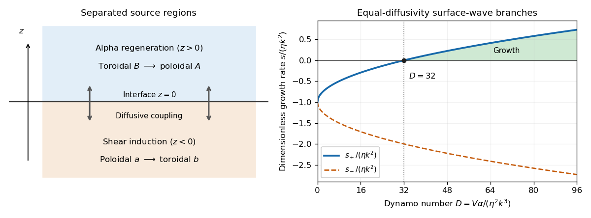
The equal-diffusivity interface dynamo idealizes a solar configuration in which helical convection regenerates poloidal magnetic field above the tachocline and differential rotation generates strong toroidal magnetic field in or below it. Diffusion communicates the fields between the two regions, closing the feedback loop. This separation is the mechanism emphasized by Parker's interface-wave model. An oscillatory traveling mode gives migrating magnetic patterns and polarity reversals; buoyant toroidal flux can appear as sunspot belts. If $x$ is a local latitude coordinate, the direction of their migration depends on the alpha–shear sign and the coordinate orientation.

The magnetic period of this branch is $2\pi /|\omega |$; polarity reverses after half a period, and activity that depends on field strength rather than sign can repeat on that half-period. This is the qualitative relation between the magnetic solar cycle and its activity cycle. The model does not itself predict the observed period or guarantee equatorward migration: those require actual geometry, transport coefficients and shear signs. Real stars also have diffusivity contrasts, meridional transport, spatially varying regeneration and nonlinear feedback. The kinematic exponential mode describes onset, while saturation and a maintained finite-amplitude cycle require further physics.