A weakly stationary process has finite second moments, a mean independent of , and a covariance depending only on the separation of the observations. Its autocovariance function and autocorrelation function arewhere the autocorrelation requires .
Write the autoregressive polynomial as , so the autoregressive model is , with the backshift operator. It is important to distinguish a weakly stationary process from a causal time series: weak stationarity alone does not require to depend only on present and past white noise.
For a two-sided weakly stationary process, the two-sided stationary inverse of an autoregressive polynomial exists and is unique if has no root on the unit circle. To find the excluded parameters, set . The imaginary part of givesThe case is harmless. The possible frequencies are . Since , and , the exceptional parameters are and . Thus, with nondegenerate white noise, the literal two-sided answer isFor completeness, away from those values has an absolutely summable Laurent series on an annulus containing the unit circle. Its bilateral coefficients define an -convergent linear filter of a stationary time series applied to , giving the required solution. Applying the same inverse to the equation gives uniqueness. At an exceptional value, the spectral measure of a stationary time series would have to satisfy . A zero of on the unit circle makes the resulting density nonintegrable near that zero, contradicting finite variance.
If the usual additional causal time series convention is intended, the causality root criterion for an autoregressive model requires the roots of to lie outside the closed unit disk. Equivalently, the roots of lie strictly inside it. The real quadratic stability conditions reduce to and , giving the narrower answerThe printed question does not explicitly impose this extra convention. Both answers have therefore been distinguished. If , the exceptional parameters permit nonunique stationary homogeneous solutions rather than the nonexistence conclusion above.
At ,Consequently the Wold representation isThe coefficients are absolutely summable, and . The past of lies in the closed linear span of the past white noise; conversely recovers that noise from present and past . Thus is orthogonal to the past of and is its one-step linear prediction error, as required for the Wold decomposition. There is no deterministic component.
Using orthogonality of the white noise, put and calculate the autocovariance by geometric sums:HenceIn particular, and ; these also satisfy the Yule-Walker equations for this autoregressive model.
Use the two-sided spectral density of a stationary process conventionThus white noise of variance has density .
Absolute summability makes the linear filter of a stationary time series well defined in : . Its mean is . For its autocovariance, continuity of the inner product givesThe sum is absolutely convergent because . It depends only on , proving weak stationarity. Inserting the spectral inversion formula and exchanging the absolutely dominated sum with the integral yieldsHere the coefficients are real, so the two factors are complex conjugates. This is the spectral density transformation under a linear filter.
Applying a second linear filter of a stationary time series givesThe composition of absolutely summable time-series filters can also be calculated directly:Indeed ; this bound also justifies the interchange of the two sums. The filter gain multiplies under this composition. The sketches for the two individual filters are:
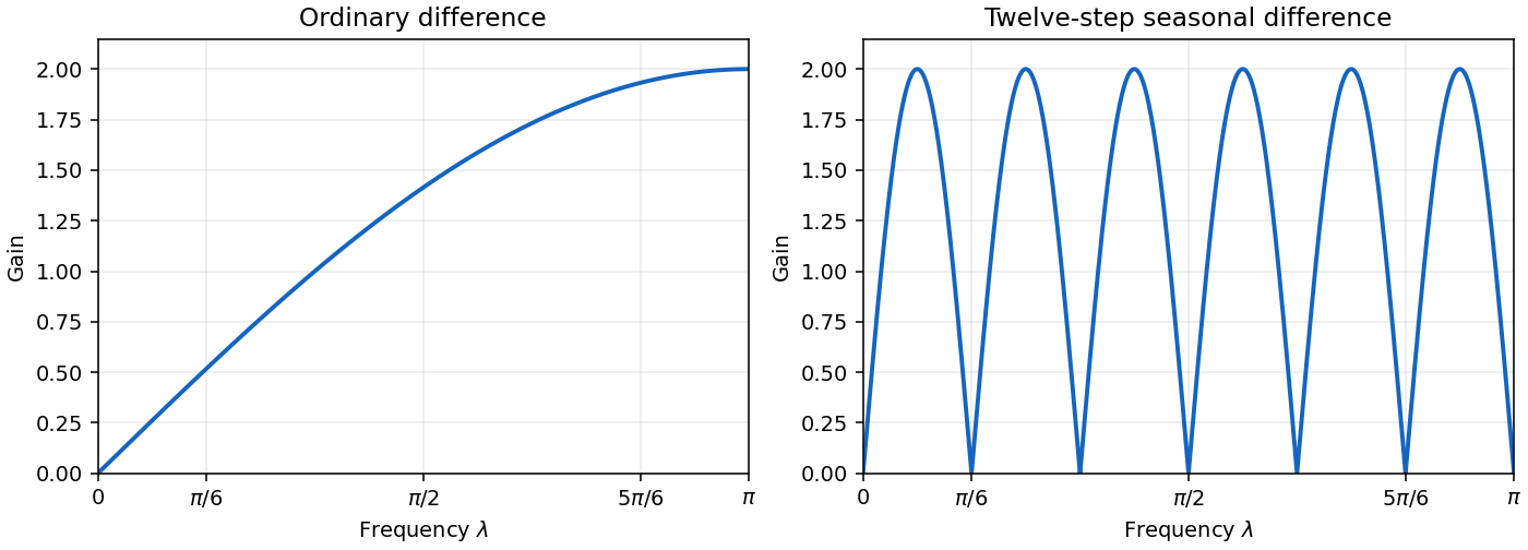
Ordinary and twelve-step seasonal difference-filter gains
. Details. 
For differencing, the only nonzero filter coefficients are and . Therefore andThe left sketch shows the filter gain increasing from zero at frequency zero to two at . This differencing filter removes a constant component and attenuates slowly varying components while relatively emphasizing higher frequencies. It is a high-pass filter, rather than an averaging or smoothing filter.
The seasonal difference operator has , and all other coefficients zero. Its frequency response is , soThe right sketch shows zeros at for , and maxima of height two at for . The seasonal difference operator removes every exactly twelve-periodic component, including a constant. Its filter gain has a comb pattern: it selectively suppresses seasonal frequencies, rather than increasing monotonically with frequency.
The composition of absolutely summable time-series filters is , with the backshift operator. Thusand its only nonzero coefficients are , , , . Multiplication of the two filter gains givesEquivalently, its spectral density transformation under a linear filter is .
A good pseudorandom number generator for Monte Carlo integration should have approximately uniform outputs, a period much longer than the intended run, and negligible detectable dependence both serially and in higher-dimensional tuples. It should be fast, reproducible from a seed, portable enough to reproduce a calculation, and numerically precise enough for the required tail probabilities. Values strictly inside avoid singularities in logarithmic inverse transform sampling. Separate simulations also need well-separated streams or seeds, rather than accidentally identical streams. A pseudorandom number generator is deterministic; these properties mean that it imitates independent uniform distributions sufficiently well for the application, not that its outputs are literally independent.
For rate , the exponential distribution has cumulative distribution function on . Inverse transform sampling gives ; since is also uniform, an equivalent answer isFor , , verifying the exponential distribution directly.
The centered Laplace distribution with density can be obtained by multiplying by an independent sign taking and with equal probabilities. Alternatively, its inverse transform sampling formula uses just one uniform variate:The first branch inverts the negative half of the cumulative distribution function and the second branch inverts the positive half. Add a location parameter if a noncentered Laplace distribution is wanted.
Correct uniformity is essential for each marginal distribution, and independence is essential for independent samples and for the sign construction. For example, setting every equal to a single uniform gives uniform marginals but identical transformed draws. Likewise, choosing a sign from the same uniform used for the magnitude can change the Laplace distribution unless the one-uniform inverse above is used.
The first algorithm uses independent normal distributions: generate with law and returnFor example, the Box-Muller transform generates two such normal variates from independent uniforms:To verify this, has density and is an independent uniform angle. Converting the resulting polar density to Cartesian coordinates gives , which factors into two independent normal distributions. Independent pairs therefore give the required sum, discarding a spare coordinate when is odd. Its moment-generating function is , that of the chi-squared distribution.
A genuinely different algorithm uses exponential-envelope rejection sampling for a chi-squared variable. Put . The target and proposal probability density functions areFor , differentiating gives , so the maximum is at . The envelope constant and normalized density ratio areThey remain valid at , where and . Repeatedly draw fresh independent , put , and accept whenThe right side is nonpositive by , so this is a legitimate acceptance probability. The joint probability of proposing and accepting in is ; conditional on acceptance the density is exactly . This proves the rejection sampling algorithm, rather than only identifying the target law.
For I prefer the second method: it reduces to a single exponential draw with no rejection. The first method is simple and attractive when normal draws are already available or is small. For larger , the second method avoids generating normals: its acceptance probability is , asymptotic to by Stirling's formula. Its expected number of proposals grows like , rather than the linear number of normal draws in the first method. Both are exact ideal-uniform algorithms; actual runtime also depends on the implementation.
For Beta sampling by gamma ratios, use either preceding chi-squared distribution algorithm to generate independent and , and returnWrite , so and . The Jacobian determinant is . The joint probability density function after this change of variables factors asIntegrating out proves the Beta distribution for .
A new method is Beta sampling by uniform order statistics. Generate independent uniforms, sort them, and return the th order statistic. There are uniforms below the selected value and above it. Selecting their labels and placing the selected observation in gives densitywhich is the Beta distribution density. The integrality of the shape parameters is what makes this order-statistic construction possible.
For jackknife resampling, calculate the leave-one-out estimates by deleting observation , and their average . The jackknife variance estimator isThe factor compensates for the small differences between the overlapping samples. For sufficiently smooth statistics it estimates their sampling variance. The related estimated bias is , leading to the jackknife bias correction .
For the nonparametric bootstrap, replace the unknown distribution by its empirical distribution functionIndependently sample observations with replacement from the original observations, compute the estimator on that bootstrap sample, and repeat this for independently generated bootstrap samples. If the resulting values are , estimate the conditional bootstrap variance byIts interpretation as an approximation to the original sampling variance relies on the bootstrap approximating the sampling law of the statistic; increasing only reduces simulation error and cannot repair a failure of that approximation.
Since the original observations are distinct, a bootstrap sample has no repeated value precisely when it contains all original values once. Of the equally likely ordered resamples, are permutations without repetition. ThereforeThe probability is zero for and rapidly approaches one as grows.
The first matrix contains the leave-one-out samples, and each element of
vect is their sample mean. For ,Thus R4a computes the jackknife variance estimator of the full sample mean:where is the unbiased sample variance. R5a computes the estimated bias used in jackknife bias correction. The identity for the average leave-one-out sample mean gives R5a = 0, apart from floating-point rounding.The second printed loop contains an indexing error: its row index is
i, although its loop variable is b. Literally, after the first block, i equals . When , every iteration overwrites row of the new matrix; the other rows remain missing. Hence vect contains one finite mean and 198 missing entries. R's default sorting removes missing entries, leaving a vector of length one, so selecting its fifth and 195th entries gives R7b = c(NA, NA). If , the matrix assignment is out of bounds; if the second block runs independently with i undefined, it fails even earlier. This is a source error, not a property of the bootstrap.Replacing just the row index by
b gives the intended algorithm: draw 199 independent bootstrap samples and sort their sample means as . The two indices are and , soThese are the endpoints of an approximate 95% percentile bootstrap confidence interval for the population mean. Their actual numerical values depend on the supplied data and random draws, which are not specified. They are not the reflected endpoints of a basic bootstrap confidence interval, and the choice of ranks does not guarantee exact finite-sample coverage.Negative covariance can be exploited through antithetic variates, but it must belong to an actual joint sampling scheme. Two separately independent samples do not inherit negative covariance merely because one can imagine a coupling of their marginal distributions. Interpret the data as independent matched pairs with covariance , together with independent unmatched observations if the sample sizes differ. Other known pairing schemes can be handled by substituting their actual covariance of the two means.
Let , , and putFor any fixed , the combination is an unbiased estimator of the common mean. Its variance is . Differentiation, or completing the square, gives the minimum-variance combination of unbiased sample means:With , both weights are positive. This is efficiency among fixed linear unbiased combinations, not a universal claim about every possible estimator for arbitrary distributions .
For an immediately implementable exactly unbiased estimator without known moments, use fixed , the pooled sample mean. Its variance iswhich shows directly the gain from negative covariance. For any fixed weight, estimate using , and using , with the usual unbiased sample covariance of the matched pairs. Substitute them into the variance quadratic. At least two matched pairs are needed to estimate their covariance nonparametrically.
If the unknown optimal weights are desired while retaining exact unbiasedness, a cross-fitted combination of unbiased sample means gives an algorithm using the supplied data. Split the independent pairs and unmatched observations into two folds, keeping each pair together and retaining observations of both types in each fold. Estimate the moments from fold 2 to choose the weight for the fold-1 sample means, adjusting the variance terms for fold 1's sample sizes; do the converse for fold 2. Clip estimated weights to , to keep them bounded when training moment estimates are unstable. Average the two held-out combinations with deterministic weights, for example one half each for balanced folds.
Conditional on its training fold, each held-out pair of sample means has expectation , and its weights sum to one. Each held-out combination, and hence their average, is therefore exactly an unbiased estimator. Under consistent moment estimation with increasing balanced folds, the weights approach and recover its first-order variance advantage. In contrast, estimating a weight from the same data to which it is applied need not yield an unbiased estimator.
Estimate the variance of this fitted-weight procedure by a bootstrap that resamples matched pairs as blocks and unmatched observations separately, repeats the entire split/weight/combination procedure, and takes the sample variance of the resulting estimates. This preserves the negative covariance and includes variability of the fitted weights. Resampling the and values independently would erase the feature responsible for the improvement. The bootstrap estimate has its usual large-sample qualification; the fixed-weight plug-in variance formula above is the simpler alternative when weights are predetermined.
A systematic Gibbs sampler updates the coordinates of successively from their full conditional distributions. At iteration , drawFor a single coordinate, if the current state has distribution , its untouched coordinates have the correct marginal law and the resampled coordinate has precisely the conditional law under . Integrating marginal times conditional therefore recovers . Each coordinate kernel preserves this invariant distribution, so their composition also preserves it. This proves the target of the Gibbs sampler; the whole systematic sweep need not be a reversible kernel.
Starting from a suitable state and assuming the required irreducibility and convergence conditions, discard an initial transient and retain subsequent states as a dependent sample from, or approximately from, . In finite-state problems irreducibility and aperiodicity suffice; in continuous-state problems the corresponding positive recurrence and ergodicity conditions must hold. Successive draws are generally dependent, so Monte Carlo uncertainty must account for that dependence.
Use the shape-scale convention for the inverse-gamma distribution: has density proportional to for . Write , , , and . The independent normal and inverse-gamma regression priors make the conditional log-likelihood plus log prior in equal, up to a constant, toDefine and . Completing the square turns this expression into plus a constant. Thus the conditional posterior distribution is the multivariate normal distributionPositive definiteness of the prior covariance matrix makes this well defined even if the design matrix is rank deficient.
Holding fixed, the factors depending on areConsequentlyThere is no additional in the shape: the normal distribution prior for is independent of . A prior scaled by would be a different model and would change that calculation.
Choose an initial . At each iteration, evaluate and using and draw from the conditional multivariate normal distribution just derived. Next compute and drawFor example, generate and set . A draw of the conditional multivariate normal distribution can be formed as with a Cholesky decomposition and a vector of independent standard normal distributions.
This two-block Gibbs sampler alternates the full conditional distributions of the independent normal and inverse-gamma regression priors posterior. The conditional-integration argument proves that its invariant distribution is the joint posterior distribution. Under the usual convergence conditions, retain the pairs after an initial transient as the requested dependent posterior sample. The new variance update uses the newly drawn coefficients, rather than the previous coefficients.
A reversible-jump Markov chain Monte Carlo calculation compares normalized model-specific densities. The fixed-order posterior written only up to proportionality in part (a) omits normalizing factors that depend on and therefore cannot simply be canceled between dimensions. Moreover, the printed question does not specify the model-order prior distribution or the probabilities of selecting birth and death moves. Denote those by , and , respectively, retaining them in the answer.
Put , , , and . The centered polynomial birth move in reversible-jump sampling changes the fitted vector by , so its new residual is . ThereforeThe map from to has ones down the diagonal and a single additional entry in the intercept row. Its Jacobian determinant is one.
Write and . The normalized multivariate normal distribution prior ratio isDivide also by the forward proposal density . The common inverse-gamma distribution prior for and the common normal-likelihood normalization cancel, since stays fixed. The forward acceptance ratio is consequentlyHere is the proposal standard deviation. If equal model priors and symmetric birth/death selection are explicitly adopted, their ratios become one; they are not determined by the PDF. The expression assumes the same hyperparameters for the variance prior in both models, as in part (a). A dimension-dependent variance prior would contribute its own ratio.
For the reverse centered polynomial birth move in reversible-jump sampling, recover from the current coefficient vector. Remove that highest-order coefficient and undo the intercept shift:No auxiliary random number is drawn for this death move: the removed coefficient supplies the auxiliary value needed to reconstruct the birth move. The reverse Jacobian determinant is also one. The inverse prediction change is , hence the residual in the lower-order model is .
Reversible-jump Markov chain Monte Carlo requires the reciprocal density/proposal ratio for the matched reverse transformation, so the death acceptance probability isExpressed directly in the current residual and the recovered lower-order parameters, this isIndeed makes this exponent the negative of the birth exponent, and all prefactors invert. Thus for matched states. This reciprocity, including the normalized prior distributions and auxiliary proposal density, gives the required detailed balance between models.
The expectation-maximization algorithm alternates conditional averaging over missing data with maximization over the parameter. Start at a parameter value for which the observed likelihood function is positive. At iteration , its E-step formsusing the current conditional law of but treating as the candidate parameter. Its M-step takesRepeat until the parameter or observed log-likelihood stabilizes. An increase of implies an increase of the observed log-likelihood: if , thenwhere Kullback-Leibler divergence is nonnegative. In general this monotonicity does not guarantee a global maximum; distinct initializations may approach different stationary points. The particular observed log-likelihood below is concave, which makes a stronger conclusion possible there.
The parameter-dependent part of the complete multinomial distribution log-likelihood isThe remaining probability factors and multinomial coefficient are constant in . If , differentiating gives , whose zero isThe log-likelihood is concave. If , its maximum is at zero; if , its maximum is at one. These boundary cases are included by the same formula. If , the data lie entirely in the parameter-independent fourth cell and every is a maximum-likelihood estimator.
Within the merged third observed cell, the probability of belonging to the original fourth cell isThe allocation therefore has the conditional binomial distributionIts conditional expectation and the filled-in missing counts arewith and .
Taking the conditional expectation of the complete log-likelihood gives the EM for merged multinomial cells E-step:This is the parameter-dependent part of . More precisely, , where the constant is independent of the candidate , interpreting factorials of noninteger filled counts through the gamma function. The expected log-factorials are not generally the log-factorials of expected counts, so literal equality including the normalization would be false. Equality up to this constant is exactly what the M-step needs. Filling in conditional means works here because the candidate-parameter terms are linear in the missing counts; it is not a universal rule for the expectation-maximization algorithm.
Initialize . At each iteration first compute by the conditional expectation above. The M-step applies the complete-data maximum-likelihood estimator to the filled counts, givingRepeat until convergence. If all counts are zero, the likelihood function is constant and any parameter can be retained. For a nonempty sample an interior start makes the displayed denominator positive.
Here the three observed cell probabilities are , and , so the observed log-likelihood isFor a nonempty sample its second derivative on isThus the maximum-likelihood estimator is unique, allowing a boundary maximum. To verify that the iteration actually finds it, let and . Then , andIf the maximum is interior, this identity moves each iterate towards it, and monotonicity of prevents crossing it. The bounded monotone iterates converge; continuity makes their limit a fixed point, and strict concavity makes that fixed point the maximum. If the maximum is at zero or one, the sign of gives the same monotone convergence towards the appropriate endpoint. In the special case , is identically one whenever its denominator is positive, so the maximum is reached in one step. An interior initialization avoids the possible spurious zero fixed point when ; starting at zero can otherwise trap the iteration even when the true maximum is positive.
Using the EM for merged multinomial cells E-step,Applying the M-step maximum-likelihood estimator to the filled counts gives
Articles by others on the same topic
There are currently no matching articles.