Past exam of the mathematics course of the University of Cambridge / 2009 / ia / Paper 2

This is a logistic equation, with positive equilibrium point $N=\alpha$ and initial population above that value. On the positive branch, put $v=1/N$. It satisfies the linear ordinary differential equation $v^{\prime }+\alpha v=1$, so $v={\alpha }^{-1}+C{e}^{-\alpha t}$. The initial condition gives $C=-1/(2\alpha )$, henceThe population decreases monotonically toward the stable equilibrium point; it never reaches it at a finite time.

The characteristic roots of the homogeneous linear ordinary differential equation are $2$ and $3$. The forcing is resonant with the $e^{3x}$ solution, so the method of undetermined coefficients uses the particular solution $x{e}^{3x}$. Thus $y=A{e}^{2x}+B{e}^{3x}+x{e}^{3x}$. The two initial conditions are $A+B=0$ and $2A+3B+1=0$, giving

With ${\sigma }_1,{\sigma }_2>0$ and $|\rho |<1$, the bivariate normal distribution has probability density functionThe strict correlation bound makes its covariance matrix positive definite, so this is an ordinary two-dimensional density rather than a distribution supported on a line.

If $\rho =0$, the bivariate normal density in part (a) factorizes asIntegrating over any product of measurable sets proves independence of random variables. Conversely, independent variables with finite second moments have $\mathbb{E}[X_1{X}_2]=\mathbb{E}[X_1]\mathbb{E}[X_2]$, so their covariance is zero and $\rho =\mathrm{Cov}(X_1,X_2)/({\sigma }_1{\sigma }_2)=0$. This proves independence of uncorrelated jointly normal variables; zero correlation alone would not imply independence without the joint normal assumption.

The events $B\cap A_i$ are pairwise disjoint and their union is $B$. Finite additivity and the definition of conditional probability therefore give the law of total probability:For the birthday problem, let $D$ mean that all birthdays differ. For $n\le 365$, sequential conditioning on previous distinct birthdays and independence of random variables giveHere each factor uses the stated bound $1-x\le e^{-x}$. For $n\ge 29$, $n(n-1)\ge 812>730\log 3$, soFor $n>365$ a match is certain by the pigeonhole principle. The threshold from the exponential bound is $(1+\sqrt{1+2920\log 3})/2\approx 28.8$, so $29$ suffices.

On an interval where $y>0$, the Bernoulli differential equation is transformed by $u=y^{1-p}$:For $f_1=1$, $f_2=x$, put $s=1-p\ne 0$. An integrating factor $e^{-sx}$ solves $u^{\prime }-su=sx$, giving $u=C{e}^{sx}-x-s^{-1}$. Thus the positive branches areon intervals where the expression in parentheses is positive. The transformation omits the separate solution $y\equiv 0$. For $0<p<1$, the right-hand side need not be locally Lipschitz continuous at zero, so nonnegative solutions can also join zero and positive branches where the original equation permits; the formula describes every strictly positive segment.

For the autonomous case, $y^{\prime }=y-{\alpha }^2{y}^p$. Its two nonnegative equilibrium points areAt the positive equilibrium point, $f^{\prime }(y_{\ast })=1-p$. If $p>1$, $f(y)>0$ below $y_{\ast }$ and $f(y)<0$ above it; hence $0$ is unstable and $y_{\ast }$ is asymptotically stable. Every strictly positive solution tends to $y_{\ast }$ forward in time.

If $0<p<1$, those signs reverse: $0$ is stable from the nonnegative side and $y_{\ast }$ is unstable. The stability at zero follows from the phase-line signs, not a finite derivative there. For initial value $0<y_0<y_{\ast }$, the transformed equation is $u^{\prime }=s(u-{\alpha }^2)$ with $s>0$. The solution reaches zero atand remains zero thereafter as a nonnegative forward solution. This is finite-time extinction in a sublinear Bernoulli equation. Initial values above $y_{\ast }$ increase without bound; the sublinear negative term prevents neither that growth nor the instability of $y_{\ast }$.

Assume $\omega >0$. The characteristic roots of the damped harmonic oscillator are $-k\pm \sqrt{k^2-{\omega }^2}$. Its general homogeneous solution isThese are respectively the underdamped, critically damped and overdamped regimes.

For the velocity-switched driven oscillator, the initial acceleration is $-{\omega }^2{x}_1<0$. Its velocity is therefore negative on the first half-cycle, and the forcing is zero:Indeed $\dot{x}=-({\omega }^2{x}_1/p)e^{-kt}\sin pt<0$ in that open interval. Set $r=e^{-k\pi /p}$; at the first turning point, $x_2=-r{x}_1$ and $\dot{x}=0$.

Put $\tau =t-\pi /p$. On the second half-cycle the velocity is positive, so the particular solution is $a/{\omega }^2$. Matching position and velocity givesIts derivative is positive for $0<\tau <\pi /p$. At the next turning point,The turning-point return map therefore repeats the initial state exactly whenThis value exceeds $a/{\omega }^2$, so the subsequent acceleration initiates the required negative-velocity half-cycle again. The switched solution is continuous with continuous velocity, and is piecewise twice differentiable; acceleration has one-sided jumps where the forcing switches.

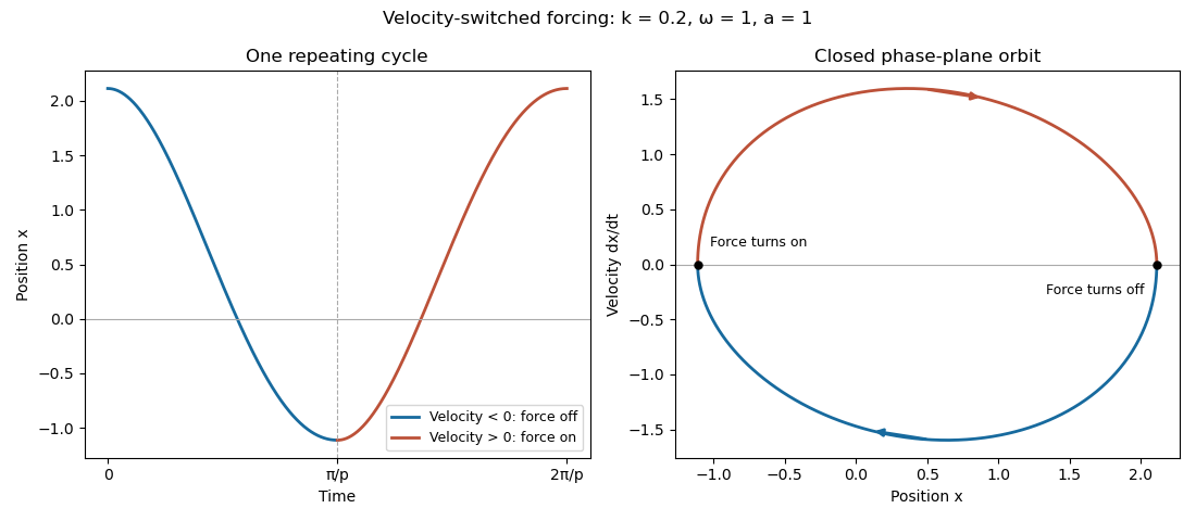
For $k>\omega$, the specified positive initial value givesThere is no next turning point: the forcing stays zero and $x$ approaches zero monotonically. The motion from the specified initial state cannot be periodic. More generally, a solution started at any positive maximum has this same obstruction; a nonconstant periodic orbit would require such a maximum. The zero equilibrium is a separate constant solution.

The origin is a regular singular point of this Kummer differential equation. Apply the Frobenius method, writing $y={\sum }_{n=0}^{\infty }{a}_n{x}^{n+r}$ with $a_0\ne 0$. The lowest power gives the indicial equationFor $n\ge 1$, comparison of the coefficient of $x^{n+r-1}$ givesSince $0<c<1$, both roots give valid independent branches. Normalize $a_0=1$:Here $(c{)}_n$ is the rising factorial, and the first series is the confluent hypergeometric function of the first kind $M(1,c,x)$. The two leading powers are distinct, proving linear independence. We describe real solutions on $x>0$, with their one-sided behavior at zero.

For the inhomogeneous equation a particular solution is $-(x+c)/2$, verified by direct substitution. Thus $y=A{y}_1+B{y}_2-(x+c)/2$. Since $y_2^{\prime }\sim (1-c)x^{-c}$, a finite derivative at zero forces $B=0$. Then $y(0)=0$ forces $A=c/2$, and the required solution isIn particular $y^{\prime }(0)=0$. The singular homogeneous branch cannot be added without violating the derivative condition.

The chain rule gives ${\partial }_x={\partial }_u+{\partial }_v$ and ${\partial }_t={\partial }_u-{\partial }_v$. Hence ${\partial }_x^2-{\partial }_t^2=4{\partial }_u{\partial }_v$, and the forced wave equation becomes $y_{uv}=1$. Integrating twice gives $y=uv+F(u)+G(v)$. At $t=0$ the initial conditions areThus $F-G$ is constant, which cancels from the final expression. Combining the remaining sum yieldsDifferentiation checks the forcing and both initial conditions.

Apply differentiation under the integral sign on the moving drop:The moving-boundary term vanishes because $h(R,t)=0$. At the origin, symmetry and regularity give $h_r(0,t)=0$. At the front, the stated $h\propto (R-r{)}^{1/3}$ gives $h^3{h}_r=O((R-r{)}^{1/3})\to 0$. Thus $\boxed{dM/dt=0}$, expressing volume conservation for this axisymmetric viscous gravity current.

With $\eta =r/t^{\alpha }$ and $R={\eta }_0{t}^{\alpha }$, substitute the self-similar solution into the conserved integral:For a nonzero finite drop volume, the power of $t$ must vanish, so $\boxed{\alpha =1/8}$. Balancing powers in the evolution equation gives the same result: its left side scales as $t^{-5/4}$ and its right side as $t^{-1-2\alpha }$. The front-edge exponent alone would not determine this spreading exponent without the conserved volume.

Use the usual assumption that the two die scores are independent random variables. A fair score has expected value $7/2$ and variance $35/12$. Linearity of expectation and the variance of a sum therefore giveCount the ordered pairs of scores to obtain the probability mass functionsOn these attainable probability supports, the maxima occur at $x=7$ and $y=0$, each with probability $1/6$; the minima occur at $x=2,12$ and $y=-5,5$, each with probability $1/36$. Outside the respective probability support, the mass is zero.

They are not independent: $Y=0$ implies equal die scores and hence $X$ is an even number, so $P(X=7,Y=0)=0$, whereas $P(X=7)P(Y=0)=1/36>0$. In fact $\mathrm{Cov}(X,Y)=\mathrm{Var}(S_1)-\mathrm{Var}(S_2)=0$: this is an example of uncorrelated random variables that are dependent.

Again assume independent die scores. Their sum has the discrete convolution of the two score distributions, soAll terms are nonnegative. The arithmetic-geometric mean inequality applied to the two extreme-score contributions givesIf all eleven probabilities were equal, normalization would make each $1/11$, but the inequality would require $1/11\ge 2/11$. This contradiction proves the sum cannot be uniform on $\{2,\dots ,12\}$, whatever the individual die probabilities.

View the accessible rooms as the open cluster of bond percolation on a rooted ternary tree. Each accessible room has three forward corridors, independently open with probability $2/3$, so its number of accessible children has the binomial distribution $\mathrm{Bin}(3,2/3)$. The counts at successive levels form a binomial branching process with offspring probability generating functionLet $q_N$ be the probability that the root has no open path to level $N$. Then $q_0=0$, and independence of the three descendant subtrees givesThe sequence increases to the smallest fixed point $q=\varphi (q)$ in $[0,1]$, the branching extinction probability. Thus $q_N$ is close to that solution for large $N$.

Connectivity is the relevant escape event: if no window is reachable, escape is impossible; if one is reachable, ordinary random wandering reaches a window eventually with probability one. Before reaching level $N$ the guest moves within a finite connected graph, so an accessible exit cannot be avoided forever. This interpretation does not require the guest to move monotonically outward.

The Galton-Watson extinction fixed point equation isIts smallest root in $[0,1]$ is $q=(3\sqrt{3}-5)/4$, not the other allowed fixed point $1$. Consequently the large-depth escape probability isFor finite $N$, the exact escape probability is $1-q_N$ and is slightly larger. Indeed ${\varphi }^{\prime }(q)=2-\sqrt{3}<1$, and the mean value theorem on $[q_N,q]$ gives $0\le q-q_N\le q(2-\sqrt{3}{)}^N$. This also quantifies how quickly the finite-depth answer approaches the displayed limit.

Integrating the uniform density gives $\mathbb{E}{X}^k={\int }_0^1{x}^{k}dx=1/(k+1)$. By independence of random variables, $\mathbb{E}(XY{)}^k=\mathbb{E}{X}^k\mathbb{E}{Y}^k=1/(k+1{)}^2$. For the remaining expected value, integrate first in $x$:The value at $y=0$ is supplied by continuity. Therefore, with the harmonic number $H_m={\sum }_{j=1}^{m}1/j$,

Conditional on one sample point being $(x,y)$, it is a maximal external point precisely when none of the other $n-1$ points falls in the upper-right rectangle $(x,1]\times (y,1]$. Its area is $(1-x)(1-y)$, so its conditional probability of being maximal is $[1-(1-x)(1-y){]}^{n-1}$. Both $1-X$ and $1-Y$ are independent uniform random variables, hence a given point is maximal with probability $H_n/n$. Summing their indicator random variables and applying linearity of expectation gives the expected number of coordinatewise maxima:This grows only logarithmically with the sample size, even though all $n$ points are potential candidates.

The law of total probability and the definition of conditional probability give Bayes' theorem:The denominator is positive because $P(E)>0$.

For the observed cargo, set $p_A=0.05$, $p_B=0.03$, $p_C=0.01$. The binomial likelihood under origin $i$ isEqual prior probabilities and Bayes' theorem make the posterior proportional to these likelihoods. The binomial coefficient cancels in the likelihood ratios:Thus $L_A/L_B\approx 4.99\times 10^{-45}$ and $L_C/L_B\approx 2.74\times 10^{-9}$, givingEven the permitted approximation $\log (1-p)\approx -p$ gives log ratios about $-93.83$ and $-23.72$, which already show overwhelming posterior preference for B. The exact logarithms are preferable because multiplication by $9800$ magnifies the approximation error. An observed contamination fraction halfway between two hypothesized rates does not give equal likelihoods: the binomial distribution assigns asymmetric probabilities to those deviations, especially at this large sample size.