Write and . The complex conjugates in the PDF giveSince , the locus is the straight line through the origin perpendicular to the position vector of in the complex plane. Equivalently,
Write . Dividing by two givesThe left side is nonnegative, so squaring is reversible only when . Squaring yields .
If , this equation implies , so the sign condition holds automatically. The locus is the parabolawith vertex at the origin, focus of a conic and directrix of a conic . Indeed the original equation equates distance from the focus of a conic with distance from the directrix of a conic on its right side.
If , the squared equation forces , making . This violates the sign condition. Thus the locus is empty for ; squaring without checking that condition would introduce a spurious parabola.
A branch of the complex logarithm must be specified to obtain a unique locus. First use the principal complex logarithm. Away from the negative real axis, write with and . Then the complex logarithms of and its complex conjugate are and . Equating real and imaginary parts gives . Consequently the principal-branch locus is the open segment of a logarithmic spiralThe origin is excluded because its complex logarithm does not exist. If the principal value is assigned argument on the negative real axis, a point there equals its own complex conjugate, so its principal complex logarithm would have to equal times itself. That forces the complex logarithm to be zero and cannot hold there; the endpoints remain excluded.
If the printed equation instead means that some values of the multivalued complex logarithms satisfy it, write those values as and , with and . Equality gives , hence , which is compatible with conjugation. Every real is allowed. Under this interpretation the locus is the entire logarithmic spiral , . The PDF does not choose between these branch conventions.
For a complex matrix, its Hermitian conjugate is obtained by transposing and taking entrywise complex conjugates:The defining conditions areFor a square matrix, either one of the two inverse identities in the unitary matrix condition implies the other. A Hermitian matrix may have complex entries, but its diagonal entries are real.
Since is an invertible matrix, so is its Hermitian conjugate, andIf is a normal matrix, substitute into the second identity to obtain , so is a unitary matrix. Conversely, if is a unitary matrix, multiply on the left by and on the right by . This gives , the defining normal matrix identity. Thus is a unitary matrix exactly when is a normal matrix.
Using the complex Euclidean norm and the normal matrix identity,Both sides are nonnegative. Therefore if and only if . This proves the stronger reusable fact that normal matrices have equal adjoint norms.
The shifted matrix is still a normal matrix, sinceand has the same expansion except that its first term is , which equals . For the given eigenvector, . Part (b), applied to , therefore gives . Since ,The corresponding eigenvalue of the Hermitian conjugate is the complex conjugate of the original eigenvalue.
Rationalizing avoids cancellation between the two large terms of the sequence:By continuity of the square root and the reciprocal at the limiting values,
Separate off the integer part of the phase. Set . Rationalization givesSince squaring removes the sign in , the given sequence satisfies . The continuity of the cosine now gives
The key fact is that convergence of a power series at one nonzero point forces absolute convergence at every smaller modulus. Indeed, if converges and , its terms form a bounded sequence, say . For ,by convergence of a geometric series.
Let be the set of moduli of points at which the power series converges, and put , allowing . The set contains zero, so its supremum is defined in . Whenever , the definition of supremum provides a convergence point with . The preceding estimate gives absolute convergence at . Whenever , convergence at would put in , contradicting its upper bound. This proves the asserted radius of convergence property, including and . Nothing in the argument decides convergence on .
For the requested boundary behavior, take the power seriesIts coefficients are for , and . At either or it is the divergent harmonic series. At either or it is , which converges by the alternating series test. In fact its radius of convergence is one, since inside the unit circle the terms are bounded by a geometric series, and outside it they do not tend to zero.
Use suffix notation, summing repeated indices from one to three. The contraction identity for the Levi-Civita symbol givesHere because is a unit vector. For the second cross product identity, use :The first term vanishes because is symmetric while the Levi-Civita symbol is antisymmetric in those indices. The last equality uses cyclicity and antisymmetry of the scalar triple product.
On the unit sphere, a great circle has radius one, so the spherical distance is its shorter arc length, equal to its central angle in . The dot product of its endpoint unit vectors is the cosine of that angle. HenceFor the angular formulas, take the ordinary nondegenerate convex minor spherical triangle: no pair of vertices is antipodal and the three vertices do not lie on one great circle. These are needed for the displayed denominators and interior angles to be defined. Merely requiring three distinct points, as the PDF does, does not exclude degeneracy.
Put , and . The outgoing unit tangent vectors at areTheir dot product is . Equivalently, they are obtained from the normalized plane normals and by the same right-angle rotation in the tangent plane: , and similarly for . Rotation preserves the dot product, givingSince and , the first proved identity becomes the spherical law of cosines:For the spherical law of sines, take norms in the second proved identity. Writing , and using , givesCyclic permutation gives the corresponding formulas at and . Dividing each by the positive product provesFinally, if all sides equal , the spherical law of cosines givesbecause makes and . Cosine is strictly decreasing on , so every angle of a nondegenerate equilateral spherical triangle is greater than .
For any linear system , a solution exists exactly when belongs to the image of a linear map represented by . If is one solution, all others are exactlysince , and conversely adding a kernel vector preserves the equation. Thus there are no solutions if , one if and , and infinitely many if and the kernel is nontrivial: every real multiple of a nonzero kernel vector gives a distinct solution. Any two solutions differ by a kernel vector. Equivalently, consistency means the augmented matrix and have equal rank of a matrix; a consistent square linear system is unique exactly when its determinant is nonzero.
For the given matrix, set and . Perform the column operation , then the row operations and . Factoring the first column givesThese operations are determinant-preserving, and the displayed polynomial identity remains valid even when a factored expression vanishes.
To find all kernels and images of a linear map, putIf is the all-ones matrix, then . The direct sum is invariant under : on it acts by multiplication by , and on by . Since , its restriction to is invertible.
For and , the kernel is and the image of a linear map is all of . Decompose the right-hand side asApplying the inverse on each invariant summand gives the unique solutionFor and , the kernel is and the image of a linear map is . A solution exists exactly when . For , all solutions areFor and , so , the kernel is and the image of a linear map is . A solution exists exactly when . All such solutions areFinally, for , the kernel is and the image of a linear map is . The right-hand side has first entry one, so there is no solution for any . These four cases exhaust all parameter values.
Let be an eigenvector of the Hermitian matrix , with eigenvalue . Multiplying by givesThe denominator is the positive real number , whileThus the numerator is real, and every eigenvalue of a Hermitian matrix is real. This argument does not require distinct eigenvalues.
Take eigenvectors for distinct eigenvalues . Since the eigenvalues are real and is a Hermitian matrix,Hence , so eigenvectors for distinct eigenvalues are orthogonal vectors. They are therefore linearly independent; after normalization the given eigenvectors form an orthonormal basis of .
Use the conventionfor the characteristic polynomial. Choosing instead multiplies it by and leaves the requested zero identity unchanged. For each eigenvector , induction gives , including . Thusbecause has the nonzero kernel vector and therefore has zero determinant. Part (a) supplies a basis consisting of these eigenvectors. A linear map vanishing on every basis vector vanishes everywhere. ConsequentlyThis proves the Cayley-Hamilton theorem identity directly in the distinct-eigenvalue case assumed here.
Expand in the orthonormal basis from part (a). ThenFor , the weights are nonnegative and sum to one. The Rayleigh quotient therefore lies between the smallest and largest eigenvalues. Conversely, normalized extreme eigenvectors give, for ,Thus the exact Hermitian Rayleigh quotient range isWhen , the range is the singleton containing the sole eigenvalue.
There is no such universal constant. For a real parameter , consider the real matrixIts characteristic polynomial is , so both eigenvalues are real and . ButFor any proposed finite , choosing violates the proposed bound. This is an explicit illustration that nonnormal eigenvalues do not bound a quadratic quotient.
Preserving the Euclidean scalar product means for every pair of real vectors . Since these bilinear expressions agree on all pairs of basis vectors, this is equivalent to : the columns of form an orthonormal basis.
The first column is a unit vector, so it is for some real . A perpendicular unit vector is one of the two choices , where . Hence all the required orthogonal matrices areHere is a planar rotation, and is determined modulo . To check the group laws explicitly, , soThis proves closure. The identity is , the inverse of is , and associativity is inherited from matrix multiplication. Thus the set is the orthogonal group .
For the Minkowski metric , preservation means for all real vectors . This is equivalent to , or, entrywise,The restriction puts the first column on the right branch of the unit hyperbola, so uniquely , for a real parameter . The third equation makes the second column a scalar multiple of : this also covers , when . The second equation makes that multiple . Thus all the required matrices areThe hyperbolic function addition formulas give , while . ConsequentlyThe product remains of the required form and its upper-left entry is positive. The identity is , and the inverse is . Together with associativity of matrix multiplication, these identities establish the group property. This is the time-orientation-preserving Lorentz group in one spatial dimension.
A member of both groups satisfies and . Multiplication of the second identity by on the left, using , gives . A real two-by-two matrix commuting with must be diagonal, since the two off-diagonal entries change sign in this equation. Its diagonal entries are by the orthogonal matrix identity, and the restriction forces the first to be . Therefore the intersection is the two-element group
Put , so . The printed summand is . If , its absolute value is at most , and the two geometric series converge. Thus there is absolute convergence.
For the series becomes , a divergent multiple of the harmonic series. For it becomesThe first series converges by the alternating series test, while the second diverges to , so their partial sums tend to . In particular, alternation of some terms does not imply convergence here. The complete classification isThere are no conditionally convergent cases.
Let . For , the absolute summand is at most , so a geometric series comparison proves absolute convergence. For , the series is : its positive term sizes decrease to zero, so the alternating series test proves convergence. Its absolute series is a divergent p-series with exponent . HenceIt converges for every real and never diverges.
For fixed real , define and . This makes exactly the summand containing nested sines. The elementary inequality gives inductivelyThe fact that an iterated contraction gives a summable orbit applies here. Comparison with a geometric series therefore givesThus the nested-sine series converges absolutely for every real ; there are no divergent or merely conditionally convergent cases.
The intermediate value theorem says that if is a continuous function, every value between and is attained at some point of .
For a proof, endpoint values are immediate, and replacing by reduces the remaining case to . The set is nonempty and bounded above; let by the least-upper-bound property. Continuity and the strict endpoint inequalities ensure : near there are points in , and near there are none. If , continuity gives a neighborhood of containing no points of , contradicting the defining approximation property of the supremum. If , continuity gives points to the right of still in , contradicting its being an upper bound. Hence , proving the intermediate value theorem.
For the distance problem, define the continuous functionIt satisfies , so it is a coercive function: as . Choose . Outside , the distance is greater than . On , the extreme value theorem gives a minimizer , with . It is therefore a global minimizer and .
For any , choose so large that . Apply the intermediate value theorem to on to obtain a point whose distance is . The distance itself is attained at , and no smaller value is possible. This is the range of a continuous coercive real function. Thus the distance set is exactlyIn particular precisely when the fixed point lies on the graph.
Rolle's theorem states that a continuous function , differentiable on with and , has for some . If is constant this is immediate. Otherwise the extreme value theorem supplies a maximum or minimum with value different from the common endpoint value, so one such extremum occurs in . At an interior maximum, the difference quotients for positive increments are nonpositive and those for negative increments are nonnegative. Their common limit, the derivative, must be zero. At a minimum the inequalities reverse, with the same conclusion. This proves Rolle's theorem.
For the two-function identity, write and , and set . This is a continuous function on the closed interval and is differentiable inside it. Its endpoint values agree:They need not be zero, but Rolle's theorem only requires equality. At the resulting point ,which proves the Cauchy mean value theorem identityFor the final endpoint limit, first state the denominator convention explicitly. In the usual zero-over-zero version of L'Hopital rule, on some whole interval ; this is understood if the displayed derivative quotient is to be a function defined throughout a deleted right neighborhood of zero. Define , making both functions continuous at zero. For , Rolle's theorem implies , since otherwise would have equal zero values at and and a zero derivative between them. Apply the proved Cauchy mean value theorem on to obtain withGiven , the hypothesis on the derivative quotient supplies such that its distance from is less than whenever . If then , so the same bound holds for . ThereforeNo continuity of the derivatives is needed.
The PDF does not explicitly state the nonvanishing condition on . If “the limit exists” permits a limit only along the natural domain where , the assertion is false, even with everywhere. The distinction concerns derivative quotient limits on partial domains. Here is a concrete counterexample to that weaker reading. Put and for . On each interval , split off the plateau . On the plateau setOn the transition interval setExtend for . The endpoints fit because , , while both and vanish at zero and one and also vanishes there. Thus are differentiable for all and tend to zero at zero. The derivative is nonzero exactly inside the transition intervals, where , so the derivative quotient has natural-domain limit zero. But , whereas . Hence has no limit. The preceding qualified proof is the intended valid form of L'Hopital rule.
A Riemann integrable function on a closed interval is bounded and has equal upper and lower Darboux integrals. More explicitly, for a partition of an interval , define the Darboux sumsThen Riemann integrability meansand this common value is the Riemann integral. Equivalently, the Riemann integrability criterion requires that for every some partition of an interval satisfies . Indeed, the common partition refinement of two partitions increases each lower Darboux sum and decreases each upper Darboux sum, so equality of the two extremal values is equivalent to arbitrarily small gaps.
Let . If the result is immediate, so take . Given , choose and the finitely many intervals supplied by the hypothesis. On each , choose a partition of an interval whose Darboux sum gap is less than , using Riemann integrability there.
Combine all these partitions with and all interval endpoints to obtain a global partition of an interval . On the chosen intervals the gaps add to less than . The complementary intervals have total lengthand on each the difference between the supremum and infimum is at most . ConsequentlyThe Riemann integrability criterion proves is Riemann integrable on . Shared endpoints cause no problem: the Darboux sums use closed intervals, and the complementary interval estimate includes every endpoint value. This proves Riemann integrability from almost full interval coverage.
Let be the set where the indicator function equals one. Fix a positive integer . Each permitted length- decimal prefix gives the intervalThere are such intervals, each of length , and they cover . Every point of is strictly inside the interval for its prefix, since its remaining tail lies between and . Thus none of the interval endpoints belongs to . The intervals are disjoint and separated: their distinct prefix integers cannot be consecutive because their final digits are only and .
The complement consists of finitely many closed intervals on which , of total length . Part (b) therefore already proves Riemann integrability, since this length tends to one.
To compute the Riemann integral directly, make a partition of an interval using and all the endpoints of the . On complementary cells the upper Darboux sum contribution is zero, and on the it is at most their total length. Moreover every nonempty cell contains a terminating decimal, which is not in : neither its terminating expansion with a zero tail nor its alternative expansion with a nine tail consists entirely of twos and sevens. Such decimals are dense, so every cell has infimum zero. ThereforeLetting gives the exact answerThis is an example of an indicator of a restricted-digit decimal set: infinitely many, indeed uncountably many, points can support an indicator function whose Riemann integral is zero.
This is a logistic equation, with positive equilibrium point and initial population above that value. On the positive branch, put . It satisfies the linear ordinary differential equation , so . The initial condition gives , henceThe population decreases monotonically toward the stable equilibrium point; it never reaches it at a finite time.
The characteristic roots of the homogeneous linear ordinary differential equation are and . The forcing is resonant with the solution, so the method of undetermined coefficients uses the particular solution . Thus . The two initial conditions are and , giving
With and , the bivariate normal distribution has probability density functionThe strict correlation bound makes its covariance matrix positive definite, so this is an ordinary two-dimensional density rather than a distribution supported on a line.
If , the bivariate normal density in part (a) factorizes asIntegrating over any product of measurable sets proves independence of random variables. Conversely, independent variables with finite second moments have , so their covariance is zero and . This proves independence of uncorrelated jointly normal variables; zero correlation alone would not imply independence without the joint normal assumption.
The events are pairwise disjoint and their union is . Finite additivity and the definition of conditional probability therefore give the law of total probability:For the birthday problem, let mean that all birthdays differ. For , sequential conditioning on previous distinct birthdays and independence of random variables giveHere each factor uses the stated bound . For , , soFor a match is certain by the pigeonhole principle. The threshold from the exponential bound is , so suffices.
On an interval where , the Bernoulli differential equation is transformed by :For , , put . An integrating factor solves , giving . Thus the positive branches areon intervals where the expression in parentheses is positive. The transformation omits the separate solution . For , the right-hand side need not be locally Lipschitz continuous at zero, so nonnegative solutions can also join zero and positive branches where the original equation permits; the formula describes every strictly positive segment.
For the autonomous case, . Its two nonnegative equilibrium points areAt the positive equilibrium point, . If , below and above it; hence is unstable and is asymptotically stable. Every strictly positive solution tends to forward in time.
If , those signs reverse: is stable from the nonnegative side and is unstable. The stability at zero follows from the phase-line signs, not a finite derivative there. For initial value , the transformed equation is with . The solution reaches zero atand remains zero thereafter as a nonnegative forward solution. This is finite-time extinction in a sublinear Bernoulli equation. Initial values above increase without bound; the sublinear negative term prevents neither that growth nor the instability of .
Assume . The characteristic roots of the damped harmonic oscillator are . Its general homogeneous solution isThese are respectively the underdamped, critically damped and overdamped regimes.
For the velocity-switched driven oscillator, the initial acceleration is . Its velocity is therefore negative on the first half-cycle, and the forcing is zero:Indeed in that open interval. Set ; at the first turning point, and .
Put . On the second half-cycle the velocity is positive, so the particular solution is . Matching position and velocity givesIts derivative is positive for . At the next turning point,The turning-point return map therefore repeats the initial state exactly whenThis value exceeds , so the subsequent acceleration initiates the required negative-velocity half-cycle again. The switched solution is continuous with continuous velocity, and is piecewise twice differentiable; acceleration has one-sided jumps where the forcing switches.
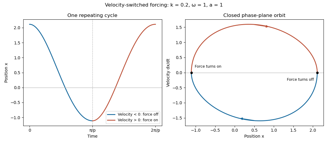

For , the specified positive initial value givesThere is no next turning point: the forcing stays zero and approaches zero monotonically. The motion from the specified initial state cannot be periodic. More generally, a solution started at any positive maximum has this same obstruction; a nonconstant periodic orbit would require such a maximum. The zero equilibrium is a separate constant solution.
The origin is a regular singular point of this Kummer differential equation. Apply the Frobenius method, writing with . The lowest power gives the indicial equationFor , comparison of the coefficient of givesSince , both roots give valid independent branches. Normalize :Here is the rising factorial, and the first series is the confluent hypergeometric function of the first kind . The two leading powers are distinct, proving linear independence. We describe real solutions on , with their one-sided behavior at zero.
For the inhomogeneous equation a particular solution is , verified by direct substitution. Thus . Since , a finite derivative at zero forces . Then forces , and the required solution isIn particular . The singular homogeneous branch cannot be added without violating the derivative condition.
The chain rule gives and . Hence , and the forced wave equation becomes . Integrating twice gives . At the initial conditions areThus is constant, which cancels from the final expression. Combining the remaining sum yieldsDifferentiation checks the forcing and both initial conditions.
Apply differentiation under the integral sign on the moving drop:The moving-boundary term vanishes because . At the origin, symmetry and regularity give . At the front, the stated gives . Thus , expressing volume conservation for this axisymmetric viscous gravity current.
With and , substitute the self-similar solution into the conserved integral:For a nonzero finite drop volume, the power of must vanish, so . Balancing powers in the evolution equation gives the same result: its left side scales as and its right side as . The front-edge exponent alone would not determine this spreading exponent without the conserved volume.
Use the usual assumption that the two die scores are independent random variables. A fair score has expected value and variance . Linearity of expectation and the variance of a sum therefore giveCount the ordered pairs of scores to obtain the probability mass functionsOn these attainable probability supports, the maxima occur at and , each with probability ; the minima occur at and , each with probability . Outside the respective probability support, the mass is zero.
They are not independent: implies equal die scores and hence is an even number, so , whereas . In fact : this is an example of uncorrelated random variables that are dependent.
Again assume independent die scores. Their sum has the discrete convolution of the two score distributions, soAll terms are nonnegative. The arithmetic-geometric mean inequality applied to the two extreme-score contributions givesIf all eleven probabilities were equal, normalization would make each , but the inequality would require . This contradiction proves the sum cannot be uniform on , whatever the individual die probabilities.
View the accessible rooms as the open cluster of bond percolation on a rooted ternary tree. Each accessible room has three forward corridors, independently open with probability , so its number of accessible children has the binomial distribution . The counts at successive levels form a binomial branching process with offspring probability generating functionLet be the probability that the root has no open path to level . Then , and independence of the three descendant subtrees givesThe sequence increases to the smallest fixed point in , the branching extinction probability. Thus is close to that solution for large .
Connectivity is the relevant escape event: if no window is reachable, escape is impossible; if one is reachable, ordinary random wandering reaches a window eventually with probability one. Before reaching level the guest moves within a finite connected graph, so an accessible exit cannot be avoided forever. This interpretation does not require the guest to move monotonically outward.
The Galton-Watson extinction fixed point equation isIts smallest root in is , not the other allowed fixed point . Consequently the large-depth escape probability isFor finite , the exact escape probability is and is slightly larger. Indeed , and the mean value theorem on gives . This also quantifies how quickly the finite-depth answer approaches the displayed limit.
Integrating the uniform density gives . By independence of random variables, . For the remaining expected value, integrate first in :The value at is supplied by continuity. Therefore, with the harmonic number ,
Conditional on one sample point being , it is a maximal external point precisely when none of the other points falls in the upper-right rectangle . Its area is , so its conditional probability of being maximal is . Both and are independent uniform random variables, hence a given point is maximal with probability . Summing their indicator random variables and applying linearity of expectation gives the expected number of coordinatewise maxima:This grows only logarithmically with the sample size, even though all points are potential candidates.
The law of total probability and the definition of conditional probability give Bayes' theorem:The denominator is positive because .
For the observed cargo, set , , . The binomial likelihood under origin isEqual prior probabilities and Bayes' theorem make the posterior proportional to these likelihoods. The binomial coefficient cancels in the likelihood ratios:Thus and , givingEven the permitted approximation gives log ratios about and , which already show overwhelming posterior preference for B. The exact logarithms are preferable because multiplication by magnifies the approximation error. An observed contamination fraction halfway between two hypothesized rates does not give equal likelihoods: the binomial distribution assigns asymmetric probabilities to those deviations, especially at this large sample size.
Articles were limited to the first 100 out of 171 total.
Articles by others on the same topic
There are currently no matching articles.