Past exam of the mathematics course of the University of Cambridge / 2014 / iii / Paper 33 (Applied Statistics)

For the normal linear model, the log-likelihood isThe full column rank of the design matrix makes $X^{T}X$ invertible. Differentiating in $\beta$ gives the normal equations $X^{T}X\hat{\beta }=X^{T}Y$. With the minimized residual sum of squares substituted, differentiation in ${\sigma }^2$ givesThese are the maximum-likelihood estimators almost surely; $RSS>0$ almost surely when ${\sigma }^2>0$ and $n>p$. The linear transformation of the multivariate normal distribution yieldsDefine the hat matrix $H=X(X^{T}X{)}^{-1}{X}^T$. The fitted values are $\hat{Y}=HY=X\hat{\beta }$, the regression residuals are $e=Y-\hat{Y}=(I-H)Y$, and $RSS=e^{T}e$. The orthogonal projection $I-H$ has rank $n-p$ and annihilates $X\beta$. By Cochran's theorem,Consequently $E({\hat{\sigma }}^2)=(n-p){\sigma }^2/n$, with bias $-p{\sigma }^2/n$. The unbiased estimator isIts square root, the reported residual standard error, estimates $\sigma$; the assertion of unbiasedness applies to the variance, not generally to its square root.

For the paper-strength analysis, let $h_i$ be the measured percentage and $z_i=h_i-\overline{h}$. Both normal linear models use independent errors of common variance ${\sigma }^2$. Their mean functions are ${\beta }_0+{\beta }_1{z}_i$ for lm1, and ${\beta }_0+{\beta }_1{z}_i+{\beta }_2{z}_i^2$ for lm2, with separately fitted coefficients. The reported residual standard errors are $11.82$ and $4.42$, respectively.

For lm1, the estimated conditional expectation at a new percentage $x$ isThe original data mean $\overline{h}$ must be used for centering the new percentage; its numerical value is not supplied in the excerpt. Because ${\sum }_i{z}_i=0$, the two columns of this design matrix are orthogonal, and $\mathrm{Cov}({\hat{\beta }}_0,{\hat{\beta }}_1)=0$. Hence the coefficient standard errors in the output giveThis estimates uncertainty in the mean. Predicting an individual future batch would additionally require the new-error variance, estimated by $11.82^2$.

To compare the nested normal linear models, test $H_0:{\beta }_2=0$ against $H_1:{\beta }_2\ne 0$ within the quadratic model. The Student t-test statistic isIts two-sided p-value is $1.89\times 10^{-8}$. Equivalently $T^2$ is a partial F-test statistic with null distribution $F_{1,16}$. Reject the linear restriction and prefer lm2 at the 5% level. Its residual spread is much smaller; the increase in the coefficient of determination from $0.3054$ to $0.9085$ supports the same conclusion, although the test is the relevant complexity-adjusted comparison.

For regression diagnostics, inspect regression residuals against fitted means and hardwood percentage for omitted curvature, a scale-location plot for nonconstant variance, and a quantile-quantile plot against the normal distribution for departures from the error assumption. Check unusual observations using regression leverage and Cook's distance, and examine residuals in collection or batch order if dependence is plausible. Independence and a common variance require substantive justification as well as these plots; a small p-value for a polynomial term does not itself check the error model.

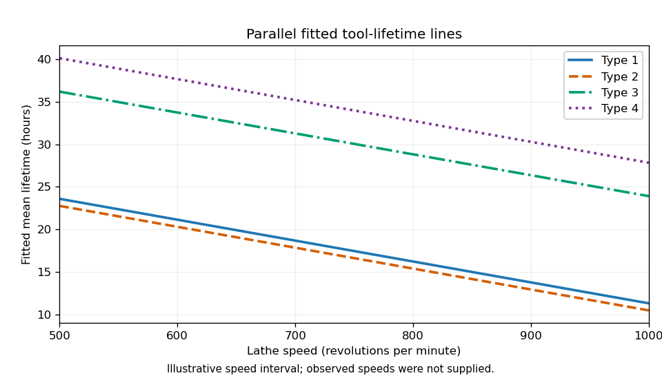
Let $s_i$ be speed and $j_i\in \{1,2,3,4\}$ the tool type. Each fit is a normal linear model with independent $N(0,{\sigma }^2)$ errors. The three mean specifications areThe constraints are treatment coding with type 1 as reference. The parameter counts are $2,5,8$, respectively. Model 2 gives parallel lines; model 3 allows interaction terms and distinct slopes.

In the analysis of variance interaction row, adding three independent slope differences costs three degrees of freedom. Its extra sum of squares is the reduction in residual sum of squares, $118.53-91.51=27.02$. Its mean square is $27.02/3\approx 9.007$, and its F-test statistic isThus the four missing entries are $3$, $27.02$, $9.01$, and $1.18$, to the precision allowed by the rounded output. This tests $H_0:{\delta }_2={\delta }_3={\delta }_4=0$ against the alternative that at least one slope difference is nonzero. Under $H_0$ and the normal linear model assumptions, the statistic has distribution $F_{3,12}$. Its p-value $0.3579213$ gives no reason to reject at 5%.

The simpler common-line model is inadequate compared with the parallel-line model. Testing $H_0:{\tau }_2={\tau }_3={\tau }_4=0$ against at least one nonzero type effect, while retaining speed, gives the partial F-testIts p-value is far below $0.001$, so reject the common-line restriction. This reduction differs from the sequential type sum of squares in the displayed table, because that table adds type before speed. Recommend model 2: different intercepts and a common decreasing slope.

The selected coefficient estimates giveThe intercept estimates the expected lifetime of type 1 at speed zero; if zero speed is outside the data range, it is only an extrapolated intercept. Its standard error is $4.039533$, and its Student t-test ratio is $8.885$, with two-sided p-value $2.31\times 10^{-7}$. At any fixed speed, type 2 differs from type 1 by $-0.833408$ hours, with standard error $1.904707$, $t=-0.438$ and p-value $0.668$, giving little evidence of a difference. Types 3 and 4 exceed type 1 by $12.607660$ and $16.539121$ hours, with standard errors $1.777937$ and $1.876116$; their test ratios $7.091$ and $8.816$ and p-values $3.68\times 10^{-6}$ and $2.55\times 10^{-7}$ support positive differences. Each of these individual coefficient tests has null value zero, alternative nonzero, and null distribution $t_{15}$.

The speed coefficient means a reduction of $0.024585$ hours per extra revolution per minute, or $2.4585$ hours per additional 100 rpm, for every type. Its standard error is $0.004682$; the ratio $-5.251$ has null distribution $t_{15}$ when the common slope is zero, and two-sided p-value $9.77\times 10^{-5}$.

The residual standard error $2.811$ estimates the common noise standard deviation in hours using 15 residual degrees of freedom, since $20-5=15$. The coefficient of determination $0.9247$ means that about $92.47\%$ of the corrected lifetime variation is explained by this fit. The overall F-test statistic $46.08$ tests the simultaneous restriction ${\tau }_2={\tau }_3={\tau }_4=\beta =0$ against at least one nonzero coefficient; its null distribution is $F_{4,15}$ and its p-value $2.974\times 10^{-8}$ rejects an intercept-only mean. These conclusions remain conditional on suitable regression diagnostics for independent, homoscedastic, approximately normal errors.

The required sketch plots the four fitted lines. Its speed interval is illustrative because the observed speeds are not supplied; the ordering and vertical gaps are determined by the fitted coefficients.

Write $\mu =\alpha /\gamma$ and $\varphi =1/\alpha$. With $\theta =-\gamma /\alpha =-1/\mu <0$, the Gamma exponential dispersion family representation iswhereSubstitution gives the original gamma density, so both unknown parameters are included. The exponential-family derivative identities yield $\mu =b^{\prime }(\theta )=-1/\theta$ and $b^{\prime \prime }(\theta )=1/{\theta }^2={\mu }^2$. ThereforeThe exact natural-parameter canonical link function is $g_{\mathrm{can}}(\mu )=-1/\mu$. The usual inverse-link convention is $g(\mu )=1/\mu$, as used by the printed R fits; multiplying the link and coefficients by $-1$ gives the natural-parameter convention. The sign convention changes neither the fitted means nor the weight matrix below.

A generalized linear model specifies independent responses in an exponential dispersion family, their means ${\mu }_i=E(Y_i)$, and a link function connecting those means to a linear predictor. In the common notation,where $a_i$ are known positive weights, $\varphi$ is the common dispersion parameter, and $V({\mu }_i)=b^{\prime \prime }({\theta }_i)$ is the variance function. The systematic part isHere $x_i$ is a row of the known design matrix and $\beta$ contains the unknown regression coefficients. The link function is invertible on the permitted mean domain; the canonical link function takes the mean to the natural parameter. This separates distributional, predictor, and link assumptions: it does not require the response itself to be normally distributed or the mean itself to be linear in the covariates.

Both fits use the same Gamma distribution mean model and inverse link function. Their coefficient estimates, fitted means and hence their weight matrices coincide: the common dispersion parameter only multiplies the likelihood score by a scalar and therefore does not change its zero. The displayed calls likewise show the same family and formula; fixing dispersion in a summary changes the uncertainty calculation, not these coefficient estimates.

For $V(\mu )={\mu }^2$ and $g^{\prime }(\mu )=-{\mu }^{-2}$, the Fisher information weights areThus the common matrix $(X^{T}WX{)}^{-1}$ is multiplied by dispersion $1$ in the exponential case and by $\hat{\varphi }=0.3103711$ in the fitted gamma case. Taking square roots of the diagonal covariances givesFor instance $0.03607\times 0.5571\approx 0.02009$ for the intercept, and the same factor applies to all the coefficients. The standard errors are smaller because the fitted dispersion parameter is below one, not because a different mean function was fitted.

For the gamma variance function, the Pearson dispersion estimator isusing $61-4=57$ residual degrees of freedom. Under a specified null dispersion ${\varphi }_0$, the scaled statistic based on squared Pearson residuals $57\hat{\varphi }/{\varphi }_0$ has an approximate ${\chi }_{57}^2$ distribution under the usual residual approximation.

Thus test1 corresponds to $H_0:\varphi =1$, equivalently gamma shape $\alpha =1$, the exponential distribution. test2 corresponds to $H_0:\varphi =1/3$, equivalently shape $\alpha =3$. The null hypotheses concern dispersion or shape, not whether the regression coefficients vanish.

The code computes lower-tail probabilities. Used as one-sided tests, the alternatives are $\varphi <1$ and $\varphi <1/3$, respectively, equivalently shapes larger than one and three. At the 5% level the first null is rejected because the lower-tail probability is $1.199504\times 10^{-7}$, while the second is not rejected because its probability is $0.3768748$. If the intended alternatives are two-sided, $\varphi \ne {\varphi }_0$, these displayed numbers must not be called two-sided p-values: doubling the smaller tail gives approximately $2.40\times 10^{-7}$ and $0.75375$, with the same decisions. The chi-squared distribution approximation is not an exact finite-sample gamma identity.

The dispersion-one assumption is strongly contradicted by the preceding calculation. Use the gamma analysis with estimated dispersion, namely the F table. A failure to reject shape three does not establish that the true shape equals exactly three; retaining the estimated dispersion parameter $0.3103711$ is appropriate.

In the analysis of deviance for nested generalized linear models, a deviance reduction for $r$ extra coefficients is divided by $r\hat{\varphi }$ when dispersion is estimated. The approximate null calibration is $F_{r,57}$. For the type term, the null is that the two type contrasts vanish, against at least one nonzero contrast. The statistic iswith approximate null distribution $F_{2,57}$ and p-value $0.02007$. For position, the null is that its coefficient vanishes after accounting for type; the statistic iswith approximate null distribution $F_{1,57}$ and p-value $0.34963$. At 5% there is evidence that component type affects the expected failure time, and no significant additional position effect. The table is sequential: the type comparison is to the intercept-only model, while the position comparison adjusts for type. The individual gamma coefficient tests also suggest that type 3 accounts for the clearer type difference. The inverse link function means its positive contrast corresponds to a lower fitted mean failure time, holding position fixed.

The three Poisson regression models have independent counts and a logarithmic link function: their mean predictors include both pc and urban in m1, only urban in m2, and only pc in m3. Nested comparisons through the full model are preferable to a direct comparison of the two nonnested one-predictor models.

To remove urban from m1, test $H_0:{\beta }_{\mathrm{urban}}=0$ against $H_1:{\beta }_{\mathrm{urban}}\ne 0$. The likelihood-ratio test statistic is the deviance differencewith approximate null distribution ${\chi }_1^2$. It is below $3.84$, so do not reject at 5%. The corresponding Wald p-value $0.588$ is consistent with this decision. To remove pc from m1, test $H_0:{\beta }_{\mathrm{pc}}=0$ against a nonzero coefficient, giving $559.17-290.64=268.53$ with approximate null distribution ${\chi }_1^2$; reject decisively. The Akaike information criterion also prefers m3, whose value $710.94$ is smaller than $712.65$ and $979.19$.

Among these three models choose m3, retaining building cover and omitting the urban indicator. This is a comparison within the stated Poisson family; its absolute fit must still be checked, as the next part does.

The chosen Poisson regression has fitted meanFor zero building cover, its fitted expected number of floods over the 25-year observation window is $e^{0.96657}\approx 2.629$. Increasing the covered proportion by $\Delta$ multiplies the fitted expected count by $e^{3.02055\Delta }$. Thus a ten-percentage-point increase, $\Delta =0.1$, multiplies the expected count by about $1.353$, an increase of $35.3\%$. A one-percentage-point increase multiplies it by about $1.0307$. The full-unit multiplier $e^{3.02055}\approx 20.50$ compares proportions differing by one, not percentages differing by one.

These are associations in the conditional expectation with the recorded final-year building cover. The regression coefficient is not automatically a causal effect of changing development, especially since the count covers 25 years while cover was measured at the end.

The residual deviance is $290.93$ on $98$ residual degrees of freedom. Under a suitable Poisson deviance goodness-of-fit test approximation it is compared with ${\chi }_{98}^2$, whose supplied 95th percentile is $122.1$. Since $290.93$ is much larger, the chosen Poisson model does not provide a satisfactory absolute fit, despite being preferred among the three candidates.

The ratio $290.93/98\approx 2.97$ suggests substantial overdispersion or mean-model misspecification. It is a deviance ratio, not the exact Pearson dispersion estimator, which cannot be computed from the excerpt. Check residual patterns, nonlinear effects, unusual rivers and dependence. A Quasi-Poisson regression could adjust uncertainty under an estimated dispersion, and a negative binomial regression could model extra count variation; a more adequate mean model may also be needed. The nominal Poisson tests in part (a) should be interpreted in light of this failure, rather than treated as a validated final analysis.

A 100-year return level is a flow threshold whose probability of being exceeded in a given year is one percent, under a stationary model for annual extremes. Equivalently, its long-run average waiting time between years with an exceedance is one hundred years. It does not imply that exceedances occur regularly one hundred years apart, or that one is guaranteed in any particular hundred-year interval. This definition uses yearly exceedance events even when the underlying observations are daily maxima.

This is the generalized Pareto distribution for the excess $X-u$, with scale $\sigma >0$ and shape $\xi$. Its support requires $1+\xi (x-u)/\sigma >0$. The Pickands-Balkema-de Haan theorem says that, for distributions in an appropriate extreme-value domain of attraction, the conditional distribution of excesses above a sufficiently high threshold approaches a generalized Pareto form. This makes it the natural peaks-over-threshold method model; it is an asymptotic justification, not an assertion that every threshold is sufficiently high.

For $\xi >0$, the tail decays as a power and has no finite upper endpoint, giving a heavy tail. For $\xi =0$, the limiting distribution is exponential, with survival probability $\exp \{-(x-u)/\sigma \}$. For $\xi <0$, there is a finite upper endpoint $u-\sigma /\xi$, giving a bounded tail. Thus the sign of the shape parameter distinguishes heavy, exponential-type and bounded tails.

In the original PDF's probability plot, most points lie close to the diagonal. The quantile plot likewise agrees well over most of the range, but the largest empirical flow, around $68.5$, is well above its fitted quantile, around $66$. The density plot captures the strongly decreasing right-skewed bulk of the excesses. The return level plot shows a broadly reasonable fit to most observations, with one conspicuously high extreme and increasingly wide uncertainty at long return periods. Consequently the generalized Pareto distribution is a reasonable first approximation, but its most extreme tail is less convincingly represented.

Reading the return-level curve at the 100-year tick givesThese are approximate graphical readings, not parameter-based calculations; rounding to whole units would give about $67$ with an interval roughly $65$ to $69$. The two blue curves are uncertainty bounds for the fitted return level, not prediction bounds for individual observations. The daily-data independence assumption and the stability of the fit as the threshold changes should be checked, for example by examining clusters of high flows and using declustering of extremes where necessary. A 100-year level also extrapolates beyond the 25-year record.

For the geometric distribution supported on positive integers, set $q=1-p$. The geometric series and its derivative giveEquivalently, the sum of the tail probabilities is ${\sum }_{k\ge 0}P(T>k)={\sum }_{k\ge 0}{q}^k=1/p$. For $p=0.02$, the expected wait is 50 years, so this is the 50-year return level. The exceedance probability determines the return period, but does not by itself determine a numerical flow rate.

Consider a competing interpolant $f$ and set $h=f-g$. At each spline knot, $h(x_i)=0$. If its second derivative roughness penalty is infinite there is nothing to prove, so assume $f^{\prime \prime }\in L^2$. Its absolutely continuous first derivative makes $h^{\prime }$ absolutely continuous as well, with $h^{\prime \prime }$ defined almost everywhere.

On each knot interval the natural cubic spline has constant third derivative. Integrating by parts once givesThe last term vanishes because $h$ is zero at both endpoints. Summing over intervals cancels the interior boundary terms, since $g^{\prime \prime }$ and $h^{\prime }$ are continuous at the knots. The exterior terms vanish because $g^{\prime \prime }(x_1)=g^{\prime \prime }(x_n)=0$. Hence $\int g^{\prime \prime }{h}^{\prime \prime }=0$. Expanding the square now givesSince $\alpha >0$, equality requires $h^{\prime \prime }=0$ almost everywhere. Absolute continuity then makes $h$ affine. It has at least two distinct zeros because $n\ge 2$, so $h=0$. The natural cubic spline is the unique minimizer. This proves the minimum roughness property with absolutely continuous first derivatives, covering the weaker regularity in the question rather than assuming competitors are twice continuously differentiable. The case of two knots is included: the minimizing spline is their straight-line interpolant.

For woman $i$, write $m_i$ for the number of births, $Y_i$ for the number with defects, $a_i$ for baseline age, and $e_i$ for exposure. Let $p_i$ be the common marginal defect probability for her births. The first fit is a grouped grouped-binomial logistic regression:It assumes independent women and, conditionally on their covariates, independent births with the same probability within each woman. The supplied birth totals are the binomial denominators; fitting the proportions with weights $m_i$ is equivalent to this grouped-binomial specification. The fitted linear predictor is $-1.74272+0.02030a_i+2.33028e_i$.

The second fit is a generalized additive model with the same logit link function and the mean specificationThe functions $f_a,f_e$ are penalized cubic regression splines with natural boundary conditions. Centering constraints such as ${\sum }_i{f}_a(a_i)={\sum }_i{f}_e(e_i)=0$ separate them from the intercept; the fitted centered intercept is $-0.2031$. Their second derivative roughness penalties control complexity.

The call estimates a common scale rather than fixing it at one. Its working variance specification for the counts isEquivalently the variance of $Y_i/m_i$ is $\varphi p_i(1-p_i)/m_i$. This is the working moment interpretation of an overdispersed binomial generalized additive model: the code uses binomial deviance for fitting and estimated scale for inference. With $\varphi \ne 1$, it is not an exact independent-binomial sampling model. Women are still treated as independent groups, but within-woman dependence or unobserved heterogeneity can motivate the extra dispersion. The quasibinomial regression interpretation states what the scaled analysis assumes without inventing a full probability distribution for its counts.

The first model's residual deviance is $671.27$ on $197$ residual degrees of freedom, a ratio of about $3.41$. This is far above the scale expected from a well-fitting dispersion-one grouped binomial regression. It suggests an inadequate mean function, overdispersion, or both. The linear age and exposure restrictions may miss nonlinear associations; the generalized additive model allows those shapes to be estimated through penalized cubic regression splines rather than assumed.

The very small exposure Wald p-value in the first fit suggests an association, but does not establish that a linear logit effect is adequate. Nor does the nonsignificant linear age term exclude every possible nonlinear age effect. Allowing estimated scale also addresses the excessive residual variation, which can arise from clustered data because several births belong to the same woman. The second model's estimated scale $3.3506$ confirms that permitting smooth means has not removed all extra variation. The reason to proceed is poor initial fit and possible nonlinear effects, with dispersion-aware inference, not merely the wish to obtain more significant tests. These observational fits alone do not establish causation by the disaster.

The trace of the smoother's influence matrix is its total effective degrees of freedom. Include the unpenalized intercept as well as both centered smooth terms:The Ref.df entries are for approximate significance calibration and must not be summed to obtain this trace. A consistency check using the generalized cross-validation form $nD/(n-\mathrm{tr}A{)}^2$ and scale estimate $D/(n-\mathrm{tr}A)$ gives $\mathrm{tr}A\approx 200(1-3.3506/3.4217)\approx 4.16$; the small difference is explained by rounding in the displayed quantities. The required trace is about $4.15$.

The original PDF's age smooth is nearly flat, its uncertainty band includes zero across the age range, and its approximate p-value is $0.859$. The exposure smooth is increasing and convex: it is fairly flat at low exposure and rises more steeply at high exposure. Its effective degrees of freedom $1.895$ suggest a modest departure from a straight line, rather than a highly oscillatory relationship.

A suitable simpler model is therefore the grouped quasibinomial regressionwith age omitted and dispersion estimated. A positive quadratic coefficient captures the convex exposure relationship; retaining the linear term respects the usual polynomial hierarchy. This model should be refitted, rather than assigning coefficients from the smooth plot. Compare its residual pattern and dispersion-adjusted fit with the additive model to check that the quadratic approximation is adequate. An exposure-only quadratic logit model is a justified parsimonious candidate, while the graph does not justify a sharp threshold or a zero-dispersion model.

Introduce a latent indicator $Z_i=1$ for a structural zero. In this parametrization $P(Z_i=1)={\pi }_i$, and conditional on $Z_i=0$ the response has a Poisson distribution with mean ${\mu }_i$. The zero-inflated Poisson regression usesIts observed probability mass function is ${\pi }_i+(1-{\pi }_i)e^{-{\mu }_i}$ at zero and $(1-{\pi }_i)e^{-{\mu }_i}{\mu }_i^{y_i}/y_i!$ at a positive count. The zero-mixing probability here is explicitly ${\pi }_i$; it is distinct from the weight of the count component.

For the expectation-maximization algorithm, start with positive ${\mu }_i$ and $0<{\pi }_i<1$. At iteration $k$, the E-step computesThis distinguishes structural zeros from Poisson-generated zeros. Up to terms independent of the new parameters, the expected complete-data log-likelihood isIt separates into a fractional-response logistic fit and a weighted Poisson fit. Because treatment is binary, each component is saturated over its two treatment groups, so the M-step has closed forms.

For $j=0,1$, let $I_j=\{i:x_i=j\}$, $n_j=|I_j|$, $S_j={\sum }_{i\in I_j}{\tau }_i$, and $C_j={\sum }_{i\in I_j}{y}_i$. The M-step score equations giveHere $\sum (1-{\tau }_i)y_i=C_j$, since every positive count has ${\tau }_i=0$. The explicit coefficient updates areIterate the E- and M-steps until the observed log-likelihood and parameter estimates stabilize. This is the EM algorithm for zero-inflated Poisson regression with explicit binary-group updates; merely naming two regression routines would not supply these expressions. Both treatment groups must be represented for both contrasts to be identifiable. Zero fitted group means or endpoint mixing probabilities are boundary solutions, interpreted through limits of the log or logit coefficients. As with other mixture models, multiple starts help distinguish competing stationary solutions; EM increases the likelihood but does not guarantee a global maximum from an arbitrary start.

There are two different effect scales in this zero-inflated Poisson regression. The count component describes the mean $\mu$ conditional on belonging to the susceptible component, including its possible zero outcomes. Its logarithmic link function coefficients exponentiate to ratios of those conditional means. The zero component describes the structural-zero probability $\pi$; its logit coefficients exponentiate to odds ratios, not probability ratios.

Holding the other covariates fixed, Centre B versus Centre A changes the susceptible count mean by the factoran increase of about $54.4\%$. It simultaneously multiplies the odds of being a structural zero byThus Centre B is associated both with higher count intensity among susceptible patients and with greater odds of belonging to the never-at-risk class.

Use no personality disorder as the reference. For women, borderline disorder multiplies the susceptible count mean by $e^{-0.224673}=0.7988$, and other disorder multiplies it by $e^{-1.564576}=0.2092$. Because the count model has sex-by-disorder interaction terms, the corresponding male comparisons must add the interactions before exponentiating:These compare men with the stated disorder to otherwise comparable men without a disorder; the female comparisons use female reference patients. The interaction multipliers $0.7865$ and $4.3157$ alone are ratios of these sex-specific disorder ratios, not the overall male disorder effects.

In the zero component there is no sex-by-disorder interaction. Borderline and other disorders multiply the structural-zero odds relative to no disorder by $0.4217$ and $0.5504$, respectively, holding centre fixed; these comparisons are the same for both sexes in the fitted zero model.

The marginal mean is $E(Y)=(1-\pi )\mu$. Therefore none of these count multipliers alone is the population-average change in expected episodes when the same covariate also changes $\pi$. For a count coefficient change $b$ and zero-logit change $g$ from baseline zero predictor $\eta$, the marginal mean ratio isFor centre use $(b,g)=(0.434635,0.6715)$; for disorder use its sex-specific count contrast and its zero contrast. This is the component and marginal effects in zero-inflated regression distinction needed to interpret these results carefully.

Let $Z=1$ mean membership in the structural-zero component. Under the fitted zero-inflated Poisson regression, $P(Y=0\mid Z=1)=1$, whereas $P(Y=0\mid Z=0)=e^{-\mu }$. By Bayes theorem, the posterior structural-zero probability isUsing the printed predictions for this patient givesThe fitted conditional probability is about $50.0\%$. It is larger than the prior fitted structural-zero probability $0.4448758$, because observing no episodes increases the probability of latent membership in that component. The interpretation “never at risk” is the model's structural class; an observed six-month zero alone does not identify the class with certainty.