The expansion is singular near the moving lower limit, so expanding throughout the original integral would lose its constant term. Introduce the symmetric exponential integralUnder , the discarded piece becomesThis is a uniform Taylor expansion because . To derive the logarithmic expansion of a symmetric exponential integral without needing another special function, first exploit the same substitution to writeThe estimate follows from . Here is Euler's constant and the small-argument expansion of the exponential integral fixes the constant as well as the logarithm.
Differentiate under the integral and integrate the derivative of over ; the exponentially small endpoint terms vanish. This gives the ordinary differential equationFor the Frobenius method at its regular singular point, write . Substitution gives and . The preceding leading calculation sets , , henceSubtracting the moving-cutoff correction to a symmetric exponential integral yields the requested answer, including the logarithmically enhanced first-order term:Thus the switchback term must be retained when asking for all contributions through order .
Set . At the positive real endpoint the contour is real and crosses the saddle point at zero. The Gaussian integral givesBoth omitted tails are exponentially small. At the negative real endpoint the contour is oriented leftward and does not cross the saddle point:The endpoint contribution in steepest descent, or one integration by parts, gives . The upper-end correction is and is much smaller. ThereforeThe sign comes from contour orientation, not from a different Gaussian convention.
Let and use the method of steepest descents with phase . For , and . The simple saddle point is : the real axis is its descending path and the imaginary axis its ascending path. The quadratic complex endpoint descent path from satisfies and can be parametrized bywith the square-root branch chosen continuously from . Increasing reduces the real part of the exponent by .
For , that endpoint path goes to positive real infinity. Deform the original contour into the real path from through the saddle point towards , followed backwards along the endpoint descent path to . The integrand is an entire function, so finite contour deformations are legitimate; connecting arcs in the far decaying sector vanish. If denotes the oriented integral from to that infinity, this givesThe last expression follows by setting : , so the endpoint integral is . This derives its phase and orientation directly.
For , the descent path from goes to negative real infinity. Deform from towards that infinity and then backwards along this endpoint path to . There is no saddle point segment, anduses the same formula with the negative square-root branch. At the contour can run from to zero and then up the imaginary axis. It gives a half-Gaussian contribution and the dominant imaginary endpoint term . The change in the subdominant saddle point contribution is a Stokes phenomenon; it does not change the leading endpoint term on either side of that angle.
The Gaussian saddle and endpoint dominance by angle follows by comparing exponential sizes and gives all fixed-angle leading behaviours:At , the endpoint term has magnitude , so the saddle point term of order still dominates. In the middle interval the endpoint term grows exponentially for , is oscillatory of order at , and decays exponentially for . On the latter interval it nevertheless decays more slowly than the fixed-endpoint term. Equality of their exponential rates means on the left half-plane, hence . At that angle both terms are required; their coefficient magnitudes are unequal, so their sum has no complete destructive cancellation.
These fixed-angle asymptotic expansions are not uniform if is allowed to vary with near a dominance transition. The endpoint/saddle balance near involves ; the two-endpoint competition near has an angular scale .
The following sketches show the contour orientations, the saddle point and both endpoints. The hyperbolic endpoint paths are followed backwards when returning from infinity to ; the dotted far-end connectors indicate the vanishing connecting arc.
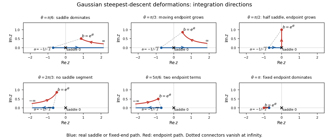
Steepest-descent contour deformations for the Gaussian integral at six endpoint angles, with saddle and endpoint paths and integration directions
. Details. 
For the matched asymptotic expansion, first determine the outer expansion. Setting away from gives , and the right boundary condition sets . At first order,soThere is no outer term: its homogeneous coefficient would be forced to zero by the right boundary condition. The logarithmic overlap forces a switchback term in the inner expansion.
Near zero, balance against to get the square-root boundary layer at a vanishing drift:For fixed expand , allowing logarithmic dependence on in . With , the leading equation is . Its bounded solutions are a constant plus an error function. The left boundary condition and the overlap value one fixThe following two solution sections complete the half-order and first-order matching; their headings retain the scaffold's organization of the supplied hints.
Write , and . The first correction in the inner expansion satisfies . Direct differentiation verifies that is a particular solution. Adding the constant and error function homogeneous solutions gives .
The left boundary condition forces . Re-expanding the outer expansion at givesTherefore , with no constant term in its large- overlap. Since and , this sets . Thus the required half-order correction isIt vanishes at zero and has the correct linear overlap. Keeping this term is essential even though the outer solution has no correction of that order.
Define the nested integralThe order- equation in the inner expansion is . The preceding result decomposes its forcing into . The particular solutions combine toFor example, follows directly by differentiating the nested integral, so the equation can also be verified without relying on the supplied particular-solution formulas. At zero ; add to impose the left boundary condition. As this givesThe outer expansion in the overlap, derived in the previous section, requires the remaining constant to be . Thus . The logarithmic matching constant is an error-function logarithmic switchback.
The complete answer through order in the inner expansion isHere , and . This expression is zero at , and its large- expansion agrees with . Together with , it covers both requested regions. The overlap uses , with the usual termwise ordering restrictions when matching higher terms.
If a single continuous approximation is desired, an additive composite expansion isThe apparent logarithmic divergence at cancels: its residual is . The composite therefore extends continuously to the left endpoint and satisfies the right boundary condition to the requested order.
For the outer expansion, the first-order reduced ordinary differential equation gives after imposing the right boundary condition. Its first correction satisfiesAn integrating factor givesThe left boundary is at , where the highest-derivative coefficient is already . Balancing that coefficient against gives a layer of width , not . This is a boundary layer around a moving endpoint:At leading order , and matching to the outer limit one while setting gives . The first correction satisfiesDirect differentiation of verifies the forcing. It vanishes both at zero and at infinity, so no homogeneous term is needed. The requested inner expansion isIts order- overlap constant is zero, agreeing with the outer expansion at the moving endpoint. The overlap can be chosen with .
An independent scaling check drops the reaction term only in the layer and integrates . Its decaying fast solution is proportional to . Sinceit gives exactly the same first correction. A useful additive composite expansion, with the left boundary value made exact, isThe exponentially small remainder at the right endpoint is beyond all retained algebraic orders.
Use the geometrical optics conventionBecause and , differentiating gives an order-one physical angular frequency and order-one physical wavenumbers. Absorb a constant leading amplitude phase into and take real; for a complex amplitude the corresponding quadratic density is .
Substitution into the wave equation gives the eikonal equation for a variable-speed wave at leading order:Choose the positive-frequency branch , ; the negative branch can be treated in exactly the same way. The imaginary first-order terms giveMultiplying by puts this wave-action transport for a variable-speed wave in conservation form:Its density is and its flux is that density times the group velocity. Independently, equality of mixed wave phase derivatives givesThis phase compatibility in geometrical optics is essential when converting the differentiated dispersion relation into equations along rays.
For completeness let be a general local dispersion relation. Define ray tracing by . Using the chain rule in and the symmetry givesLikewise cancels its advective term because . Hence the Hamiltonian ray equations for a local dispersion relation areThe derivatives on the right hold the wavevector fixed. For this wave equation they reduce to
When , the ray invariants are and , while . For a monochromatic component with these fixed invariants write , soUsing the stated independence of from , the wave-action transport for a variable-speed wave becomes . ThereforeThis is the stationary wave amplitude in a stratified wavespeed; is the constant for that component or ray family.
At the proposed simple turning point of a variable-speed wave, take and . On the chosen positive branch this entails . DefineAs the ray approaches from below, andThe amplitude diverges and the vertical group velocity vanishes. The WKB approximation also fails its slow-variation condition when . The turning-point enhancement of wave amplitude shows that this divergence is a failure of the outer ray approximation, rather than an actual infinite solution.
To derive the inner wavefield directly, separate the conserved horizontal wave phase and frequency in the original differential equation:Dividing by gives . Set . The second derivative is of size , whereas , so the Airy scaling at a variable-speed wave turning point isThe first-derivative term is smaller by , and higher coefficients in the expansion of give the same relative order. Thus the general leading inner profile is a linear combination of the two Airy functions and . For decaying Airy continuation and ray reflection, if the physical continuation is bounded and decays into , its growing coefficient is zero. In that usual evanescent continuation the wavefield has the formWithout a condition in the evanescent region the corresponding term remains admissible locally; the given existence of a wavefield below the turning point alone does not select its coefficient.
Finally, the outer amplitude at distance is for and fixed nonzero . The oscillatory Airy turning-point connection formula has exactly the same envelope on the allowed side. Therefore the inner wavefield has magnitude . The decaying Airy continuation matches an incident and reflected pair of rays, so a single upward branch must be supplemented by its reflected branch near the turning point; no formal coefficient matching is needed to identify this magnitude.
Articles by others on the same topic
There are currently no matching articles.