For the two-zone cloudy annulus transmission model, assume a uniform stellar disc, an opaque planet below , , and constant total slant optical depth within each radial zone. Neglect scattered light entering the beam and the planet's own emission. A ray transmits the fraction , so each zone blocks its projected area multiplied by .
The opaque disc, cloudy annulus and clear annulus have areas , and , respectively. Thus the exoplanet transmission spectrum, expressed as total transit depth, isHere means the total optical depth on rays assigned to the cloudy zone. If it denotes cloud extinction alone, its exponent must instead contain the sum of cloud and gas optical depths. For a geometrically thin exoplanet atmosphere, the two atmospheric prefactors become and .
An opaque exoplanet cloud deck gives the simpler expressionThe exoplanet cloud deck raises the wavelength-independent occulting radius and suppresses the clear atmospheric contribution. If , the spectrum is flat at ; if , the ordinary annulus model for transmission spectroscopy is recovered. Stellar limb darkening and varying tangent-ray optical depth would require an intensity-weighted radial integral rather than this constant-depth model.
Assume an isothermal atmosphere in hydrostatic equilibrium, with constant gravity , mean molecular weight , and an ideal gas equation of state. Use for the atmospheric scale height, to distinguish it from the total observable height . Thenso the cloud-top pressure in an isothermal atmosphere isAn opaque, approximately grey exoplanet cloud deck can flatten the exoplanet transmission spectrum if the remaining gas above it has little wavelength-dependent extinction. If its top nearly reaches the observable atmospheric extent, , this gives . More generally, a top at atmospheric scale heights has ; illustrative values and give and .
A flat exoplanet transmission spectrum and alone do not determine a unique cloud-top pressure. The temperature, gravity, mean molecular weight and cloud altitude, or equivalent opacity information, are also needed. A large mean molecular weight can itself suppress spectral features, so the exoplanet cloud deck interpretation is conditional.
Assume that the optical continuum is dominated by Rayleigh scattering by particles much smaller than the wavelength, and that their column abundance is fixed. Their cross-section, hence the slant optical depth, scales as . Differentiating the annulus model for transmission spectroscopy exactly gives the logarithmic slope of total transit depthFor and , the slope lies between and zero, but generally depends on wavelength. In the optically thin limit, , so its slope is . It vanishes as the atmospheric signal becomes negligible compared with the opaque disc; it also approaches zero in the saturated optically thick limit.
The familiar value applies to the optically thin atmospheric excess,or formally to a model in which is negligible. For an ordinary thin exoplanet atmosphere, however, , so neglecting the opaque planetary baseline in the total transit depth is not usually justified. A universal for the logarithm of the total transit depth does not follow from the stated model.
In a stratified isothermal atmosphere, the related scattering slope of a transmission spectrum is instead , obtained by moving the effective tangent level to keep its slant optical depth of order unity. Consequently there. The radius slope, atmospheric-excess slope and total-depth slope are different observables.
This is a semi-grey irradiated atmosphere in radiative equilibrium. The quantities have these meanings:
- is the local atmospheric temperature.
- is the internal effective temperature of a planet, defined by the upward intrinsic flux .
- is the irradiation temperature, conventionally , so is the incident substellar bolometric stellar flux.
- is the stellar flux redistribution factor. With albedo treated separately, uniform global averaging gives and dayside averaging gives . If reflected power is included, the absorbed factor is reduced accordingly; these choices must not be double-counted in .
- is the downward thermal optical depth, measured from the top with mean infrared opacity .
- is the ratio of the mean stellar-band absorption opacity to the mean thermal opacity, not the gas's adiabatic index.
The model assumes a static plane-parallel atmosphere, separate grey stellar and thermal bands with constant opacities, local thermodynamic equilibrium for thermal emission, negligible scattering, and transport by radiative transfer rather than convection. The Eddington closure approximation sets the thermal angular-moment ratio to , and the upper boundary supplies the usual term. Treating the incoming radiation with representative direction cosine gives its attenuation . Intrinsic flux enters from below, while the imposed external stellar flux is absorbed from above.
With constant gravity and hydrostatic equilibrium, , allowing conversion to an atmospheric pressure-temperature profile. This last relation additionally assumes constant thermal opacity. The grey treatment describes the energy balance approximately; it does not resolve individual molecular absorption lines.
The thermal optical depth increases inward, so an atmospheric thermal inversion requires . Differentiating the semi-grey irradiated atmosphere profile givesTherefore the inversion criterion with intrinsic planetary flux isAn inverted layer exists at the top precisely whenFor , it extends overprovided the logarithm is positive. Otherwise the profile has no inverted interval. For a strongly irradiated hot Jupiter, and the threshold is approximately ; the intrinsic flux eventually restores an inward-increasing temperature at greater depth.
Large visible absorption opacity deposits stellar heat high in the exoplanet atmosphere. Gas-phase titanium monoxide and vanadium monoxide are candidate absorbers in sufficiently hot layers. An atmospheric cold trap or other condensate loss can remove them, while sufficiently high temperature and vigorous mixing can help keep them in the gas. The condition concerns absorbing opacity: highly reflective scattering alone does not deposit the required heat.
For uniform composition, the Schwarzschild criterion gives stability against convection whenA parcel displaced upward expands approximately adiabatically. If the ambient logarithmic temperature gradient is shallower than the adiabatic temperature gradient, the parcel cools more than its surroundings, becomes denser, and sinks back. Equality is neutral stability; a steeper gradient drives buoyant growth.
For a diatomic ideal gas with active translational and rotational degrees of freedom, and . If the infrared opacity is constant, , so the profile's radiative temperature gradient isAn atmospheric thermal inversion has negative and is stable by this criterion. Composition gradients require the Ledoux criterion; molecular dissociation and changing heat capacities can also change the numerical adiabatic temperature gradient.
Take to increase inward, so the positive coefficient describes an inward-increasing temperature. Constant gravity and hydrostatic equilibrium give , henceMatching the radiative temperature gradient to the adiabatic temperature gradient gives the formal local boundary relationThe same result follows from radiative diffusion: for constant upward thermal flux and Rosseland mean opacity , .
There is an important limitation to treating as constant over the entire radiative layer. Integration from an irradiated outer boundary givesFor a diatomic ideal gas, , so this profile cannot actually reach a radiative-convective boundary. Formally, imposing a constant would givewhich is positive only for . A finite boundary for a normal molecular atmosphere requires additional opacity, flux, or thermodynamic variation. The local matching formula is usable near a real boundary, but constant is not a complete global model of it. This is the convective stability of a constant-opacity irradiated atmosphere.
For the intended order-of-magnitude scaling, suppose the local values of and are comparable for Jupiter and a hot Jupiter, and assume scales with planetary equilibrium temperature. Equal absorbed-flux factors around the same stellar luminosity give . Taking and a representative close-in orbit yieldsThis illustrates how irradiation can push a boundary much deeper. It is a conditional estimate calibrated from the supplied reference, not a self-consistent prediction of the globally constant- model. Different intrinsic cooling flux, opacity, gravity, or atmospheric metallicity of a giant planet can substantially alter it.
Four mechanisms that can produce disequilibrium chemistry in an exoplanet atmosphere are:
- Atmospheric photochemistry. Stellar ultraviolet photons initiate reactions whose products need not follow local thermochemical equilibrium. The ozone layer on Earth is a solar-system example. Calculations for HD 189733 b predict enhanced hydrogen cyanide and acetylene from the processing of methane and ammonia; these are model examples rather than assertions of an unambiguous detection.
- Vertical transport and chemical quenching. When the eddy mixing time is shorter than the chemical relaxation time, gas retains a deeper abundance above its chemical quench level. The excess carbon monoxide in Jupiter's cool atmosphere exemplifies carbon monoxide–methane quenching. Models of HD 189733 b predict quenched methane and ammonia abundances differing from their local chemical equilibrium values. The enhancement or depletion depends on the underlying atmospheric pressure-temperature profile.
- Horizontal chemical quenching. If the atmospheric advection time is short, winds move chemically processed gas into regions with different irradiation or temperature faster than it can re-equilibrate. Transport of gas within Earth's ozone layer moves material away from its local photochemical production regions. Models of HD 209458 b show that dayside carbon monoxide-rich composition can persist into the cooler nightside instead of forming the local chemical equilibrium amount of methane.
- Condensation with sedimentation or rainout. Finite-rate cloud formation can depart from phase equilibrium, while atmospheric condensate rainout removes elements from a layer and changes its gas composition. Earth's water atmospheric cold trap limits the supply of water to the stratosphere. In HD 209458 b models, titanium-bearing condensates can settle and suppress upper-atmospheric titanium monoxide. The remaining gas can still be in local chemical equilibrium with its depleted inventory: rainout is an open-column effect, not necessarily a failure of equilibrium among all gas reactions.
The exoplanet transport and photochemical examples follow kinetic atmosphere calculations and models including horizontal transport; the condensate example is examined in cold-trap calculations.
Take the logarithm to base ten and write pressure in units of , so its argument is dimensionless. Continuity of the atmospheric pressure-temperature profile givesThusIf the logarithm means , the equivalent constant is . A plot of temperature against logarithmic pressure is vertical in each isothermal region and straight between the two endpoints.
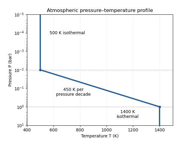
Atmospheric pressure-temperature profile
. Details. The processes can be organized by the supplied pressure ranges, although the exact boundaries require reaction rates, irradiation and mixing information:
- At , the dense gas can approach thermochemical equilibrium because collisions and reactions are relatively rapid. Deep carbon monoxide and molecular nitrogen can provide reservoirs for transported material.
- At , the falling temperature slows chemical conversion. Vertical transport can produce a chemical quench level when the chemical relaxation time crosses the eddy mixing time. Horizontal chemical quenching is also possible if dayside and nightside conditions differ. Suitable species can condense and undergo atmospheric condensate rainout where a saturation curve is crossed.
- At , slow thermal chemistry permits a quenched atmospheric mixing ratio to survive. Atmospheric photochemistry can dominate where stellar ultraviolet photons penetrate, often at still lower pressures; atmospheric haze may form from its products. Extremely high layers can also experience atmospheric escape.
The profile identifies plausible chemical regimes, but does not fix their transition pressures by itself. In particular, cloud formation depends on the species-specific condensation curve, and ultraviolet processing depends on shielding.
For solar elemental abundances, take a molecular hydrogen- and helium-dominated atmosphere with atmospheric carbon-to-oxygen ratio near . The principal oxygen-bearing molecule is generally water; the carbon and nitrogen carriers depend on both temperature and pressure.
At the cool observable upper layers, methane is the expected main carbon reservoir under chemical equilibrium, with abundant water and much less carbon monoxide. At the hotter layers approaching , carbon monoxide becomes the main carbon carrier and water contains much of the oxygen not bound in it. The relevant law of mass action follows fromLower temperature favors the exothermic methane-forming direction, while increasing pressure favors the side with fewer molecules. This explains why the change of dominant carrier cannot be specified by temperature alone.
Nitrogen is distributed between molecular nitrogen and ammonia. Cooling favors ammonia, but low pressure favors molecular nitrogen; it is therefore unsafe to call ammonia dominant throughout the low-pressure region. The exact partition requires the equilibrium constant for .
Carbon dioxide is usually a minor constituent at solar composition; hydrogen cyanide and acetylene are much less abundant than the principal carbon carriers in this oxygen-rich equilibrium case. Condensation can remove refractory species where a condensation curve is crossed. The robust cool-atmosphere expectation is a molecular hydrogen–helium background with methane and water, changing toward carbon monoxide in hotter layers. Precise mixing ratios require thermodynamic data and an explicitly specified elemental inventory after rainout.
Four possible molecular signatures of disequilibrium chemistry in an exoplanet atmosphere, measured through an exoplanet transmission spectrum or exoplanet emission spectrum, are:
- Excess carbon monoxide in the cool upper layers, where local chemical equilibrium would place most carbon in methane. This can indicate carbon monoxide–methane quenching from deeper hot gas.
- Suppressed methane bands relative to the same cool equilibrium model, consistent with transport preventing complete carbon monoxide conversion or with photochemical loss.
- An ammonia abundance inconsistent with the local equilibrium nitrogen partition, potentially recording nitrogen–ammonia quenching. Its direction must be evaluated for the actual atmospheric pressure-temperature profile; a depleted value is possible when hotter, molecular nitrogen-rich gas is transported upward.
- Enhanced hydrogen cyanide or acetylene bands, consistent with atmospheric photochemistry acting on the transported carbon and nitrogen reservoirs.
The first two signatures can be consequences of the same process and are not independent evidence for two mechanisms. Changes in atmospheric carbon-to-oxygen ratio, atmospheric metallicity of a giant planet, exoplanet cloud coverage, and the atmospheric pressure-temperature profile can mimic abundance changes. A convincing inference compares several molecular bands with a chemically consistent equilibrium model rather than identifying one unusual band alone.
At fixed temperature and pressure, the atmospheric carbon-to-oxygen ratio controls the division of the elemental inventory among carbon monoxide, methane, water and other molecules. For an oxygen-rich mixture, water can remain after carbon monoxide consumes its share of oxygen. Increasing the atmospheric carbon-to-oxygen ratio reduces the oxygen available for water, particularly in the hotter layers where carbon monoxide is stable. Near or above unity there, water can become strongly depleted while excess carbon feeds methane, hydrogen cyanide and acetylene. This familiar hot carbon-rich behavior should not be applied unchanged to every cool layer: at , methane formation can leave substantial water even at high atmospheric carbon-to-oxygen ratio.
Increasing the atmospheric metallicity of a giant planet at fixed elemental ratios increases the heavy-element inventory relative to molecular hydrogen and helium. Abundances of water and the major carbon-bearing molecules generally rise while molecular hydrogen remains dominant. In that regime, the law of mass action for givesWhere carbon monoxide and water each scale roughly linearly with enrichment , carbon dioxide consequently scales approximately as . This scaling changes when molecular hydrogen ceases to dominate or chemical partitioning changes. Higher enrichment can also favor carbon monoxide over methane at fixed conditions, increase mean molecular weight, and reduce the atmospheric scale height and transmission-feature amplitudes. Cloud formation and atmospheric condensate rainout alter the observable elemental ratios relative to the bulk ones.
Use the standard local chemical quench level approximation: carbon monoxide-rich gas from the hot deep region is transported upward, and conversion becomes slower as the gas enters the cooler layers. Assume that neither a faster loss process nor strong compositional fractionation removes carbon monoxide above the quench level. For an effective mixing length , the eddy mixing time is , so outrunning conversion near requiresThe usual order-of-magnitude choice is , the local atmospheric scale height at . Equal planetary mass and radius give the same gravity as Jupiter; with the same mean molecular weight, the atmospheric scale height scales linearly with temperature. To use the supplied reference, additionally adopt a representative Jovian reference temperature . ThenUsing directly with and Jovian gives and , the same order of magnitude. The supplied Jovian height is approximate and does not specify its reference temperature. Inserting unchanged for the hot gas would instead give and neglect this temperature scaling.
The pressure separation is relevant to a stronger, whole-column transport estimate. With constant gravity and mean molecular weight, the profile givesIf one additionally requires diffusion through the entire column within , a sufficient conservative condition is . It is not a necessary local quench condition: the chemical relaxation time is expected to become much longer in the cooler gas, so a longer total transit time can still preserve carbon monoxide.
The usual quench estimate is of order under the stated scale-height assumptions. A unique bound for survival to cannot be inferred from one reaction time without assumptions about its variation, the mixing length and upper-atmospheric losses.
Three observational signatures constrain exoplanet atmospheric dynamics:
- A displaced maximum of the exoplanet thermal phase curve. If the thermal maximum precedes exoplanet secondary eclipse, the hottest region is displaced east of the substellar longitude in the usual synchronously rotating geometry. The observed offset for HD 189733 b is consistent with eastward heat advection and atmospheric superrotation; the early infrared phase-curve measurement established this effect.
- Warm nightside emission and a reduced day-night contrast. The amplitude of an exoplanet thermal phase curve constrains day-night heat redistribution. For HD 189733 b, the same observations found hemisphere brightness temperatures roughly and , supporting substantial transport to the nightside instead of purely local reradiation.
- Atmospheric line shifts after orbital motion is removed. A residual Doppler shift measures winds projected along the line of sight. A carbon monoxide signal blueshifted by roughly in HD 209458 b was interpreted as day-to-night winds in high-resolution transit spectroscopy. Rotational broadening and different limb velocities can supply additional dynamical information.
Opacity, exoplanet cloud distributions, and pressure-dependent brightness temperature affect the phase-curve interpretation. These measurements constrain circulation through atmospheric models; a single offset or line shift does not uniquely determine a three-dimensional wind field.
The geometric albedo compares the planet's reflected brightness at full phase with that of a perfectly reflecting Lambertian surface in the form of a flat disc of the same projected area, illuminated by the same incident flux. The Bond albedo is the fraction of total incident stellar power reflected in all directions and over all wavelengths. They need not be equal: the planetary phase integral and the incident spectral weighting connect them.
For a blackbody star, the incident flux at orbital distance isAssume negligible intrinsic luminosity, thermal emissivity one, and efficient day-night heat redistribution giving uniform emission over the whole planet. The absorbed and emitted powers areUsing the Stefan–Boltzmann law gives the planetary equilibrium temperatureFor a representative emitting area encoded by a stellar flux redistribution factor , the equivalent expression iswith for global uniform emission and for uniform dayside-only emission. The Bond albedo, rather than the geometric albedo, belongs in the energy budget. Internal heat, wavelength-dependent emissivity and imperfect redistribution require corresponding modifications.
Use the single-layer greenhouse model with a blackbody surface and one isothermal atmospheric layer. The layer is transparent to incoming stellar radiation, absorbs a fraction of the surface's thermal radiation, and has the same thermal emissivity by Kirchhoff's law of thermal radiation. Here , and is the planetary equilibrium temperature defined by the absorbed global stellar flux . Neglect convection, latent heat transport and intrinsic heat.
The layer absorbs and emits upward and downward. For , its energy balance givesThe surface receives the absorbed stellar flux plus downward atmospheric emission, soEliminating yieldsThe outgoing top-of-atmosphere flux is , confirming overall energy conservation. At , and the decoupled layer's temperature is not determined; at , . This warming is the restriction of thermal escape by the absorbing and emitting layer.
A mass-radius curve of solar-composition substellar objects must specify age, irradiation and composition. For a mature, weakly irradiated hydrogen–helium sequence, the qualitative mass-radius relation has three main trends:
- At low giant-planet masses, weak compression allows a rough scaling at nearly fixed mean mass density. Radius rises toward a broad maximum around one to a few Jupiter masses.
- Through massive gas giants and brown dwarfs, radii remain near Jupiter's and eventually decline as compression and electron degeneracy pressure become important. A nonrelativistic degenerate stellar polytrope gives the approximate polytropic mass-radius relation ; finite thermal pressure and real equations of state flatten and modify this idealized scaling.
- Above the hydrogen-burning minimum mass, sustained hydrogen burning supplies the energy that supports a rising low-mass main-sequence branch. For near-solar composition, the threshold is around Jupiter masses (about solar masses), with composition-dependent variation. Red dwarfs then have radii increasing with mass, approximately linearly over part of the low-mass sequence.
The conventional deuterium-burning mass near Jupiter masses marks a commonly used giant-planet/brown dwarf classification scale, not a sharp discontinuity in radius or a universal formation boundary. Young brown dwarfs are larger and cool by contraction; irradiation, a heavy-element core and hot-Jupiter radius inflation shift planets away from a single solar-composition curve.
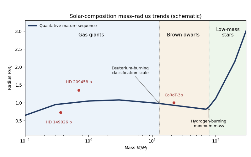


The drawing is a qualitative mature sequence, not an interpolation of a specified evolutionary model grid. Three relevant observations, using representative historical measurements, are:
- Inflated radii: HD 209458 b has a radius around at a mass around , illustrating hot-Jupiter radius inflation relative to a simple mature unirradiated sequence. Early transit photometry measured its unusually large radius.
- Compact metal-enriched planets: HD 149026 b was measured near and . Its small radius for its mass and irradiation implies substantial heavy-element enrichment in interior models, showing the importance of composition in the planetary mass-radius relation; see the discovery analysis.
- Jupiter-like sizes at substellar masses: CoRoT-3b was measured near but only , supporting the broad near-constant-radius region extending into brown dwarf masses. Its measured mass and radius also illustrate why mass alone does not establish a formation history.
Gas-giant radius growth gives way to a nearly Jupiter-sized compressed branch, followed by rising radii in hydrogen-burning stars.
Three major research directions, appropriate to the scientific questions posed in 2018, are:
- Characterizing small-planet atmospheres and habitability. Measure an exoplanet transmission spectrum and an exoplanet emission spectrum to establish whether rocky planets retain atmospheres, determine their composition and climate, and test exoplanet habitability. Interpreting an exoplanet biosignature requires a planetary and stellar context: photochemical false positives, exoplanet cloud obscuration and atmospheric escape can all affect apparently promising molecules.
- Connecting atmospheres and interiors to planet formation. Combine planetary mass-radius relations with ages, host-star abundances, atmospheric metallicity of a giant planet and atmospheric carbon-to-oxygen ratio to test growth and migration histories. Exoplanet interior-composition degeneracy, chemical processing and atmospheric condensate rainout prevent a molecular abundance or bulk radius from being a unique record of birth conditions.
- Understanding atmospheric circulation and thermal evolution across populations. Combine exoplanet thermal phase curves, Doppler spectroscopy and pressure-dependent spectra to test day-night heat redistribution, exoplanet cloud formation and disequilibrium chemistry in an exoplanet atmosphere. Relate these measurements to hot-Jupiter radius inflation, internal cooling and atmospheric escape, using comparative observations to distinguish mechanisms instead of fitting each planet in isolation.
These are research goals rather than claims that the relevant mechanisms or habitable atmospheres have already been established.
Articles by others on the same topic
There are currently no matching articles.