Past exam of the mathematics course of the University of Oxford / 2021 / Prelims / Mathematics V resit (A10142W1)

Source: released examination PDF, bundle pages 274–278.

Use polar coordinates with $0\le r\le {\sin }^2\theta$ and $0\le \theta \le \pi$. The Jacobian determinant gives $dA=rdrd\theta$, so the area isThe trigonometric identityreduces the integral to its constant term: both cosine terms have zero integral over this interval. Therefore

Write the centroid as $\overline{\mathbf{r}}=\overline{x}\mathbf{i}+\overline{y}\mathbf{j}$. The region has reflection symmetry in the $y$-axis: replacing $\theta$ by $\pi -\theta$ changes $x$ to $-x$ and preserves $y$ and $dA$. Thus symmetry in integration givesFor the other first moment of area, use $y=r\sin \theta$ in polar coordinates:Here the last integral has the value allowed in the paper. Dividing the first moment of area by the area found in i givesThe positive vertical coordinate agrees with the fact that the entire region lies above the $x$-axis.

Express the position vector in the suggested orthonormal basis as $\mathbf{r}=X{\mathbf{e}}_1+Y{\mathbf{e}}_2+Z{\mathbf{e}}_3$. ThenThis orthogonal transformation preserves $x^2+y^2+z^2=X^2+Y^2+Z^2$ and has Jacobian determinant of absolute value one, so $dV=dXdYdZ$. The basis actually reverses orientation; the absolute value of the Jacobian determinant is why no minus sign enters the volume integral. Also $x-y=\sqrt{2}Z$, so the half-space becomes $Z\ge 1/2$.

At each fixed $Z\in [1/2,1]$, the section is the disk $X^2+Y^2\le 1-Z^2$, of area $\pi (1-Z^2)$. Its reflection symmetry in $X$ makes the integral of $X$ vanish. Hence the required triple integral isThe negative sign is also consistent with the cap lying in the direction $(1,-1,0)$, where its average $y$ coordinate is negative.

One sufficient version of the divergence theorem is the following. Let $R$ be a bounded region in ${\mathbb{R}}^3$ with a closed, piecewise smooth surface as its boundary, and let $\mathbf{F}$ be a continuously differentiable function with values in ${\mathbb{R}}^3$ on an open neighbourhood of the closure of $R$. With $\mathbf{n}$ the outward unit normal vector,The boundary surface integral is the total outward flux integral. If the boundary has several components, each has the outward orientation relative to the material of $R$; inner components therefore point into the holes. Edges and isolated vertices may be omitted when assigning the unit normal vector, since they have zero surface area.

For each of the three constant Cartesian unit vectors ${\mathbf{e}}_j$, apply the divergence theorem to the vector field $\varphi {\mathbf{e}}_j$. Its divergence is ${\partial }_j\varphi$, soThese are precisely the three components ofThus the volume integral of the gradient is the boundary surface integral weighted by the vector surface element $d\mathbf{S}=\mathbf{n}dS$. The regularity needed here is that $\varphi$ be continuously differentiable on a neighbourhood of the closure of $R$.

Use cylindrical coordinates $(\rho ,\theta ,z)$. The right circular cone is described by $0\le z\le 1$ and $0\le \rho \le a(1-z)$, and the divergence of $\mathbf{F}=(0,0,z^2)$ is $2z$. Direct integration gives

To check the boundary flux integral independently, first consider the base $z=0$. Its outward unit normal vector is $-\mathbf{k}$, but $\mathbf{F}=0$ there, so its flux is zero. Parametrize the lateral surface byThe cross productpoints outward: its horizontal component points away from the axis of the cone. This gives the vector surface element without separately normalizing it. Consequently the lateral flux integral isAdding the zero base contribution agrees with the volume integral, verifying the divergence theorem. The apex has zero surface area; the vector field is smooth there, so no additional flux is hidden at that point.

The curl isTo establish that $\mathbf{F}$ is a conservative vector field, construct a potential of a conservative vector field directly:This gradient calculation is valid on all of ${\mathbb{R}}^3$, and hence also on the cone. The explicit potential of a conservative vector field supplies the required global justification.

Let $\Sigma$ be a compact, piecewise smooth oriented surface with piecewise smooth boundary, and let $\mathbf{F}$ be continuously differentiable on an open neighbourhood of $\Sigma$. The Stokes theorem statesThe boundary orientation must agree with the chosen unit normal vector by the right-hand rule. For an upward orientation on a horizontal disk, its boundary is traversed counterclockwise when viewed from above. Reversing the orientation reverses both the line integral and the surface integral.

Choose the outward unit normal vector on the upper hemisphere. The curl of $\mathbf{F}=(4y,x,2z)$ isIn spherical polar coordinates, putHere $n_z=\cos \phi$ and $dS=a^2\sin \phi d\phi d\theta$. The surface integral is thereforeThe compatible boundary orientation follows increasing $t$ in $\mathbf{r}(t)=(a\cos t,a\sin t,0)$, $0\le t\le 2\pi$. On this circle,Thus the line integral iswhich agrees with the surface integral as required by the Stokes theorem.

Use the outward orientation on the unit hemisphere and counterclockwise boundary orientation on the unit circle. With $\mathbf{r}(t)=(\cos t,\sin t,0)$ and $f=x=\cos t$, the vector line integral isFor the surface integral, $\nabla f=\mathbf{i}$ and the outward unit normal vector is $\mathbf{n}=(x,y,z)$, since the radius is one. The cross product isThe integral of $y$ is zero by reflection symmetry. Using the same spherical polar coordinates as in ii, with $a=1$, the other component isHenceverifying the vector-valued Stokes identity directly, component by component. The wedge symbol in the paper denotes the cross product here.

Choose the scalar fieldThe allowed vector-valued Stokes identity givesEvery boundary point lies on the unit circle in the $xy$-plane, so $f=1/2$ throughout the boundary. Since the line integral of $d\mathbf{r}$ around a closed curve is the zero displacement,Only the boundary value of this scalar field mattered: the interior of the surface need not be part of a sphere. Either consistent choice of orientation gives the same zero answer.

The Fourier cosine series and Fourier sine series use the respective formsTheir Fourier coefficients, obtained from Fourier orthogonality, areIn particular the constant term is $a_0/2={\pi }^{-1}{\int }_0^{\pi }f(t)dt$. The Fourier cosine series is the Fourier series of the even extension $f(|x|)$, made $2\pi$-periodic. The Fourier sine series is the Fourier series of the odd extension, equal to $f(x)$ for $0<x<\pi$ and $-f(-x)$ for $-\pi <x<0$, again made $2\pi$-periodic.

The theorem on pointwise convergence of a piecewise smooth Fourier series gives the average of the two one-sided values of the corresponding periodic extension. Under the usual piecewise smooth interpretation of the paper's derivative assumption, the even extension is continuous at $0$ and at the joined endpoints $\pm \pi$. ThusFor the odd extension, the values on either side of zero are $-f(0)$ and $f(0)$; those on either side of $\pi$ are $f(\pi )$ and $-f(\pi )$. ThereforeThe endpoint values are also immediate because each sine term vanishes there. If $f(0)$ or $f(\pi )$ is nonzero, the Fourier sine series does not reproduce that endpoint value. Merely assuming that the derivative is locally piecewise continuous in the open interval would be weaker than the usual piecewise smooth hypothesis; the convergence assertion uses the standard endpoint regularity implicit in that hypothesis.

For the Fourier cosine series, integration by parts givesand, for $n\ge 1$,Only odd Fourier harmonics remain, so

For the Fourier sine series, another integration by parts givesConsequentlyAt $x=0$ and $x=\pi$, the Fourier sine series instead has value zero.

To describe the requested graphs precisely, take $t\in [-\pi ,\pi )$ congruent to $x$ modulo $2\pi$. The Fourier cosine series converges to the continuous triangular periodic extensionIts minima occur at the even multiples of $\pi$, with value $1$, and its maxima at the odd multiples, with value $1+\pi$. The Fourier sine series converges toThe jump discontinuities at even multiples of $\pi$ go from $-1$ to $1$; those at odd multiples go from $1+\pi$ to $-(1+\pi )$. Each jump is assigned its midpoint, zero, by the Fourier series.

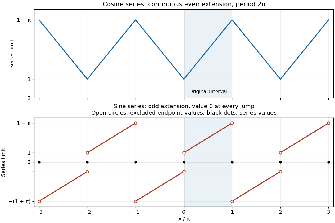
The truncated Fourier cosine series gives the better approximation on the closed interval, in the senses of uniform convergence and the asymptotic L2 norm error. To make the comparison precise, let $C_N$ and $S_N$ retain the frequencies $1\le n\le N$, with the constant term also included in $C_N$.

The cosine Fourier coefficients are $O(n^{-2})$. In fact, absolute convergence gives the uniform tail boundFor the Fourier sine series, every Fourier partial sum satisfies $S_N(0)=S_N(\pi )=0$. Thusso there is no uniform convergence to $f$ on the closed interval. Its odd extension has jump discontinuities, producing the Gibbs phenomenon near the endpoints; its Fourier coefficients decrease only like $1/n$.

The advantage persists in the L2 norm, which ignores individual endpoint values. By Parseval's identity and Fourier orthogonality,The nonzero odd cosine coefficients and both parity classes of sine coefficients also give matching lower bounds of these orders by comparison with the corresponding p-series. Hence their L2 norm errors decrease respectively like $N^{-3/2}$ and $N^{-1/2}$. This is a comparison of approximation quality in specified norms, not a claim that one finite sum has smaller error at every individual interior point.

Take $\boxed{f(x)=\sin x}$. This function is not a polynomial: it is nonzero and satisfies $f^{\prime \prime }=-f$, whereas a nonzero polynomial cannot satisfy that identity, since taking two derivatives reduces its degree or gives zero.

By Fourier orthogonality, the Fourier sine series consists of the single term $\sin x$. Thus every truncation with $N\ge 1$ is exact, including at the endpoints. In contrast, using the product-to-sum trigonometric identity in its Fourier cosine coefficients givesFor example, ${\int }_0^{\pi }\sin x\cos (2mx)dx=-2/(4m^2-1)$ follows by integrating the two resulting sine terms. Therefore the Fourier cosine series isEvery finite cosine truncation omits infinitely many nonzero Fourier coefficients, so Parseval's identity gives it strictly positive squared L2 norm error. The one-term sine representation has zero error in both the L2 norm and the supremum norm, proving the requested advantage.

Treat the boundary data as $2\pi$-periodic in the angular variable. Denote the outer data by $g(\theta )$, and set $h(\theta )=f(a,\theta )$ for the inner data. Define their mean and nonconstant Fourier coefficients byThe outer data have reflection symmetry, so all their sine Fourier coefficients vanish. Their mean is $1/2$, and their cosine Fourier coefficients are

The angular Fourier harmonics for a single-valued harmonic function in an annulus are $\cos (n\theta )$ and $\sin (n\theta )$, with integer $n\ge 1$. Their radial factors are independent combinations of $r^n$ and $r^{-n}$; the zero angular mode has radial factor $A_0+B_0\log r$. For arbitrary inner data, the sine and cosine modes need independent radial coefficients: forcing them to share one radial factor, as in the product form supplied in the paper, would impose an extra restriction. For either sine or cosine mode, if its outer and inner coefficients are $v$ and $w$, the radial coefficients $\alpha ,\beta$ obeySolving this linear system givesIt is convenient to collect the result into the annular harmonic interpolation factorsThey satisfy $H_n(1)=1$, $H_n(a)=0$, $K_n(1)=0$ and $K_n(a)=1$. The zero mode satisfies $A_0=1/2$ and $B_0=(p_0-1/2)/\log a$. Therefore the required separation of variables solution isAll dependence on $f(a,\theta )$ is given by the displayed integrals. Substituting $r=a$ leaves its Fourier series, and substituting $r=1$ leavesthe Fourier series of the specified outer step. The radial factors satisfy $r^2{R}^{\prime \prime }+r{R}^{\prime }-n^{2}R=0$, so each nonconstant term satisfies Laplace's equation; $1$ and $\log r$ do also. For integrable boundary data the radial factors give exponential decay on every closed subannulus strictly inside $a<r<1$, justifying the necessary termwise partial derivatives there.

There is a qualification at the two outer jump discontinuities. By pointwise convergence of a piecewise smooth Fourier series, the outer series gives $1/2$ at $\theta =\pm \pi /2$, whereas the printed data assign $1$ at those two points. Thus the displayed solution attains the outer data at their continuity points, and has radial limit $1/2$ at the jumps. One may separately assign the boundary value $1$ at the two exceptional points without changing the interior harmonic function, but no continuous extension can match the discontinuous data there. For piecewise smooth inner data, the analogous boundary trace agrees with $h$ at continuity points and with its midpoint at jumps. Some regularity of $h$ is necessary for a classical interpretation; the problem imposes none explicitly.

Put $u(r,\theta )=R(r)\Theta (\theta )$ in Laplace's equation and multiply by $r^2/(R\Theta )$ on intervals where the factors are nonzero. Separation of variables givesand henceThe angular Dirichlet boundary conditions are $\Theta (0)=\Theta (\pi /2)=0$. Multiplication of the angular equation by $\Theta$, followed by integration by parts, givesFor a nonzero angular eigenfunction this forces $\lambda >0$: equality would make $\Theta$ constant and then zero. Write $\lambda ={\mu }^2$. The first angular condition removes the cosine term, and the second requires $\sin (\mu \pi /2)=0$. ThusThe radial Cauchy-Euler equation has the two solutions $r^{2n}$ and $r^{-2n}$. By superposition, the general separated series is thereforeThe coefficients are arbitrary subject to convergence with enough partial derivatives on compact subsets to give a harmonic function and to the prescribed zero values on the two open radial edges. Completeness of the sine eigenfunctions gives the usual series representation for solutions smooth up to those edges on closed radial subintervals. There is no constant or logarithmic zero mode because its angular factor would be linear in $\theta$ and would vanish at both ends only if it were zero.

The negative powers must be retained: the stated domain omits $r=0$, and no boundedness at that vertex is prescribed. For example, $r^{-2}\sin (2\theta )$ is a harmonic function satisfying both edge conditions. An additional boundedness condition as $r\to 0$ would remove all $B_n$; an additional value on the circular arc would then determine the remaining $A_n$. With only the conditions in the paper, neither restriction is available and the solution is not unique.

Let $u_1,u_2$ be two solutions with the same data, and write $w=u_1-u_2$ on the rectangle $\Omega =(0,\pi )\times (-1,1)$. By linearity,The normal derivative is $-w_x$ on the left edge and $w_x$ on the right edge, so it vanishes on both. The energy method applies Green's first identity, which follows by integratingIt givesThe boundary term vanishes on each horizontal edge because $w=0$, and on each vertical edge because ${\partial }_{n}w=0$. The interior term vanishes because $w$ is a harmonic function. Since the continuous integrand $|\nabla w{|}^2$ is nonnegative, a zero integral forces $\nabla w=0$. The rectangle is connected, so $w$ is constant; its zero value on either horizontal edge makes that constant zero. HenceThis proof assumes enough boundary regularity for Green's first identity. It also works in the finite Dirichlet energy class using the weak identity with test function $w$, so it remains applicable when corner derivatives are not continuous. It proves uniqueness conditional on existence and does not impose a compatibility condition for arbitrary $f,g$.

Set $u=X(x)Y(y)$ in Laplace's equation. Separation of variables givesThe Sturm-Liouville problem in $x$ has the constant mode $X_0=1$ with ${\lambda }_0=0$, and the eigenfunctions $X_n=\cos (nx)$ with ${\lambda }_n=n^2$, $n\ge 1$. Indeed, integration by parts makes $\lambda$ nonnegative; for $\lambda >0$ the first Neumann boundary condition removes the sine term and the second requires $\sqrt{\lambda }$ to be an integer. For $\lambda =0$, both derivative conditions make $X$ constant.

Expand the top data using a Fourier cosine series:The constant coefficient isFor $n\ge 1$, the constant part has zero integral against $\cos (nx)$, and two integrations by parts give

Since the bottom value is zero, a convenient factor depending on $y$ for the nonconstant modes is $\sinh (n(y+1))$, which vanishes at $y=-1$. Its value at $y=1$ is $\sinh (2n)$. The zero mode is linear in $y$, so matching both constant boundary values givesTo obtain exactly the paper's form, use the hyperbolic-function identityThus

Each product of hyperbolic sine or hyperbolic cosine with $\cos (nx)$ has $u_{xx}+u_{yy}=0$. The zero mode is also a harmonic function. On $-1\le y\le 1$, the factor $\sinh (n(y+1))/\sinh (2n)$ lies between zero and one. Since $\sum n^{-2}$ converges, the Weierstrass M-test gives uniform convergence on the closed rectangle. The series therefore gives zero at the bottom and the continuous Fourier cosine series of ${\pi }^2-x^2$ at the top, including its endpoints. On compact subsets with $y<1$, the factors decay exponentially with $n$, justifying termwise partial derivatives. In particular $u_x=0$ on both open vertical edges because every differentiated cosine factor vanishes there. The solution has finite Dirichlet energy: Fourier orthogonality gives the $n$th nonconstant mode's energy as $(\pi /2)n{g}_n^2\coth (2n)=O(n^{-3})$, whose sum is finite. Here $\coth$ is the hyperbolic cotangent. Thus a proves uniqueness in that class.

There is a corner compatibility condition for mixed boundary data in the printed wording. The top data have $g^{\prime }(\pi )=-2\pi$, but the paper writes $u_x(\pi ,y)=0$ even at $y=1$. The series solves the interior equation and all the open-edge boundary conditions; the literal derivative condition at $(\pi ,1)$ is incompatible with the top data. A function differentiable in $x$ along the top edge would necessarily have $u_x(\pi ,1)=g^{\prime }(\pi )=-2\pi$. Hence it cannot simultaneously satisfy the printed zero derivative at that corner, and there is no solution with all those literal corner requirements. The standard interpretation of this mixed boundary condition imposes the Neumann boundary condition on the open sides and the Dirichlet boundary condition continuously on the horizontal edges. Differentiating the series term by term on the top edge would be invalid at this corner; the uniform convergence of the undifferentiated series does not license that operation.