On its specified domain of admissible functions, a self-adjoint operator equals its adjoint, including the adjoint domain. Its integration identity on the interval isFor a differential operator, the boundary conditions must make the boundary form from integration by parts vanish. Formal symmetry of the differential expression alone does not specify a self-adjoint boundary-value problem.
Apply this identity to two eigenfunctions. Since the weight is real,First take : positivity of shows , so the eigenvalues are real. For distinct eigenvalues, subtraction therefore givesThis is orthogonality of Sturm-Liouville eigenfunctions in the weighted inner product, rather than necessarily in the unweighted inner product.
To obtain Sturm-Liouville form, multiply the equation by . The derivative identitygivesThe weight determines the weighted inner product on . It is integrable but singular at the endpoints, where also vanishes. Thus this is a singular-endpoint Sturm-Liouville problem, not a regular problem with strictly positive endpoint values of . The transformation in part (ii) specifies its admissible Dirichlet realization; these are the Dirichlet eigenfunctions of the Chebyshev differential operator.
Let for . The chain rule givesSubstitution cancels the first-derivative terms and leaves . The endpoint conditions become . For , the first condition selects , and the second requires . Thus a nonzero solution requires an integer . The case gives and both conditions force it to vanish. Negative integers give the same eigenvalues and eigenfunctions up to sign, so take .
For vector normalization, use :Choosing a positive real normalization constant givesHere is the Chebyshev polynomial of the second kind. The factors make both endpoint values zero. The derivatives need not stay finite there; instead has finite endpoint limits, ensuring that the relevant boundary form vanishes.
Using the normalized eigenfunctions and the same change of variables, their weighted inner product isFor distinct positive integers , the product-to-sum identity givesbecause each integrated sine has integer-multiple-of- endpoints. For , the integral is one by the normalization already calculated. HenceThis verifies orthonormality explicitly, with the Kronecker delta.
Put for separation of variables. Multiplication by givesSingle-valuedness requires a -periodic angular function. The nonzero possibilities are for integers . For , is a combination of and , while the radial Euler-Cauchy equation has solutions . At , periodicity excludes an angular term proportional to , and gives .
Superposing the separated harmonic functions yieldsTo obtain the general solution, expand any sufficiently regular harmonic function in a Fourier series on circles; each Fourier coefficient satisfies the corresponding radial equation. The coefficients must give the required convergence on compact annuli. Because no condition at zero or infinity is imposed in this part, neither radial branch is discarded.
Boundedness at the origin allows only for nonconstant interior modes; decay at infinity allows only outside. Write the common surface potential in its Fourier series as , where . Continuity then makes the corresponding interior and exterior factors and .
Their outward radial derivatives at the surface are inside and outside. Thus the jump is . Equating it to minus the prescribed surface-charge mode givesTherefore the potential of a charged cylindrical shell with angular Fourier data isEither branch gives the same value at . The mean angular mode is zero: outside, neither a constant nor a logarithm can survive the condition at infinity; continuity then forces the interior constant to zero. Consequently .
The absence of a mean term in the surface charge density is essential. A nonzero mean would require a logarithmic exterior potential and would be incompatible with decay at infinity in this two-dimensional reduction. The normalization follows the stated derivative jump, with no additional permittivity factor introduced.
Use the product rule for the vector field :The mixed dot products cancel. Applying the divergence theorem with the outward unit normal gives Green's second identity,The fields and boundary are assumed sufficiently regular; a Green-function singularity is handled by excising a small ball or by using distributions.
Fix inside and put in Green's second identity. The volume integral becomesHere Laplace's equation eliminates the second term, and the Dirac delta evaluates the first. Reversing the signs in the boundary integral givesAll boundary derivatives act on the integration variable , not on the fixed evaluation point .
Impose the homogeneous Dirichlet boundary condition on the boundary variable:This removes the term containing the unknown normal derivative of . The prescribed boundary values alone then determine the solution throughFor an unbounded domain one also imposes the appropriate decay condition at infinity. This defines the required Dirichlet Green function.
Let the evaluation point be , , and reflect it to . The method of images constructsThe two Euclidean distances coincide on the plane, so there. The negative image source lies outside the domain; inside, only the real source contributes to . The difference also decays at infinity.
On the plane write and set . The outward unit normal of the upper half-space is . Direct differentiation givesSubstituting into the boundary representation from part (c) yields the Poisson kernel for the upper half-space:Its sign is positive, as expected from the maximum principle for nonnegative boundary data. Its normalization can be checked in polar coordinates:As the kernel is an approximate identity, recovering at its continuity points. Boundary data must have the decay and regularity compatible with the stated condition at infinity.
On the axis, the Poisson kernel for the upper half-space depends only on the radial boundary coordinate. Integrating over the disk givesTherefore the axial Poisson extension of a circular boundary patch isIt tends to one as the axis approaches the boundary inside the patch, and tends to zero as far above it.
The boundary values jump at the circular rim. They are understood almost everywhere, or as limits at continuity points; changing the assigned value on that measure-zero circle does not change the integral. At a rim point the vertical limit is one-half, rather than a continuous extension with the specified value on both sides of the jump.
Let be meromorphic on and inside a positively oriented simple closed contour , with finitely many isolated poles inside and none on . The residue theorem statesThe positive orientation is counterclockwise. A clockwise contour reverses the sign, and the residue is the coefficient of in the local Laurent series.
The denominator vanishes at the four roots of , namely for . They are simple poles, since is nonzero at each root and the numerator does not vanish there. The simple-pole residue formula givesExplicitly,There are no branch points or other finite singularities. At infinity the function is , so infinity is removable rather than a pole.
Close the interval with an upper semicircle, traversed counterclockwise. On its large arc,so the estimation lemma bounds the arc integral by . The enclosed residues are those at and , whose sum is . The residue theorem therefore givesThe positive sign agrees with the nonnegative real integrand.
Choose a branch of the complex logarithm with , placing its branch cut down the negative imaginary axis. Thus for , while on the negative real axis for .
Integrate around an upper semicircle, with a small clockwise semicircular indentation above zero. The large arc contributes , and the small arc contributes . The only enclosed pole is , withWriting for the required integral, the negative real segment contributes . Hence the residue theorem givesThe imaginary terms cancel, leavingThe integral converges at both endpoints because is integrable near zero and is integrable at infinity. As a real-variable check, scaling reduces the result to the vanishing first logarithmic moment at , one of the logarithmic moments of the Cauchy kernel.
Use the Fourier transform convention . For a transformable response with the necessary boundary terms vanishing, integration by parts givesTransforming the differential equation therefore gives , soThe identities also hold for tempered distributions. The denominator factors as ; its two poles are in the upper half-plane, corresponding under inverse factor to the causal Green function of a damped oscillator.
The frequency-domain formula selects the Fourier-transformable response. Decay of the force alone would not remove arbitrary homogeneous solutions, which grow towards negative time and do not have an ordinary bilateral Fourier transform.
Substitution givesThe inverse Fourier transform is . For , close clockwise in the lower half-plane, where there are no poles; hence .
For , close counterclockwise in the upper half-plane. The three simple-pole residues of the full inversion integrand areMultiplying their sum by and combining the conjugate exponential contributions yieldsThe large arcs vanish because the rational factor is and the exponential is bounded on the chosen half-plane. At zero, the right-hand value and first derivative are both zero, matching the negative-time branch, so no unwanted delta or delta derivative appears in the second-order equation.
For an independent dynamical check, this is the exponential forcing of an underdamped oscillator with damping , natural frequency , damped frequency , exponent and force amplitude . For positive time its substitution gives .
The result of part (i) vanishes identically on the open interval , so its first and second derivatives also vanish there. Substituting into the equation of motion immediately givesThus the force has no negative-time prehistory, consistent with the causal Green function of a damped oscillator. In fact, direct inversion or the positive-time substitution above identifies ; the given numerator corresponds to a negative exponential force with this Fourier convention. Here is the Heaviside step function; its value exactly at the jump does not affect the transform.
Preserving Cartesian lengths and Euclidean inner products requires an orthogonal matrix:Its determinant is . Relative to an originally right-handed frame, gives a right-handed frame and a left-handed frame. More generally, this sign determines whether the two frames have the same or opposite orientation.
The tensor component transformation law isFor a tensor field, the components are compared at the same physical point, whose coordinates satisfy .
Define the symmetric tensor and antisymmetric tensor parts by and . The transformed transpose satisfies . Thereforeand similarlyBoth obey the tensor component transformation law. Thus the symmetric and antisymmetric parts are themselves second-order tensors. Taking a transpose and forming linear combinations commute with this orthogonal change of frame.
Let . Averaging each pair of transposed entries gives the symmetric tensorFor , the upper block is the outer product of with itself. It sends that vector to times itself and annihilates its perpendicular. Thus its orthonormal principal axes and corresponding eigenvalues areTaking these vectors as the rows of the change-of-components matrix givesThis matrix is orthogonal with determinant one. These are the principal axes of a planar rank-one tensor block.
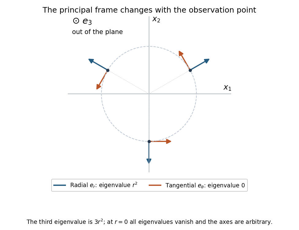
The radial and tangential principal directions rotate with position; the third principal axis is perpendicular to this plane
. Details. 
The matrix is a pointwise frame transformation: because its angle varies with position, it does not represent one fixed Cartesian rotation diagonalizing the entire field everywhere. On the axis , the symmetric tensor is zero; all principal values coincide and any orthonormal axes may be chosen. The displayed formula for is therefore used only off that axis.
The scalar, symmetric-traceless and axial tensor decomposition fixes the scalar part by the trace:Subtracting this isotropic part from the symmetric tensor in part (c) givesIts trace is zero. The antisymmetric tensor part isAdding reconstructs every entry of .
Subtracting a scalar multiple of the identity preserves every eigenvector: if , then . Thus the principal axes are the same as in part (c), with shifted principal valuesThe two tensors are coaxial symmetric tensors. At both vanish, so neither specifies unique axes.
Take downward vertical distances from the support. The climber positions are , and . Their kinetic energy is thereforeIntegrating the tension-extension relation gives the elastic potential energy for each taut rope. Because downward displacement lowers gravitational potential,An arbitrary additive constant in is immaterial. This is the vertical-motion model implicit in using only rope lengths as generalized coordinates; swinging angles are not additional degrees of freedom in this model.
The Euler-Lagrange equations giveFor example, differentiating with respect to collects contributions from all three climbers, because changing moves all of them. At equilibrium, all accelerations vanish, soThe top rope supports the total weight, while each lower rope supports only its own climber. These extensions are positive, consistent with the taut-rope tension law.
Set . The equilibrium equations cancel the constant gravitational and elastic terms, leaving the small-oscillation mass and stiffness matricesThe off-diagonal mass terms arise because rope-length coordinates are not absolute climber displacements. For any nonzero velocity vector, , so is a positive-definite matrix.
Within the vertical Hookean model, the displacement equations are exactly linear while all ropes stay taut. Small amplitudes ensure that none reaches the slack regime .
Exchange symmetry of climbers 2 and 3 gives , for which . HenceThe physical displacements are , so climber 1 is stationary and the other two move vertically with equal amplitudes in opposite directions. Their changes in force on climber 1 cancel.
For the remaining symmetric modes, put and let . The eigenproblem becomes , . Eliminating gives . Therefore . Since ,For clarity, their relative physical climber displacements, rather than rope-length amplitudes, areThe lower mode moves all climbers in phase; the higher mode moves the lower pair against the top climber. These are the normal modes of three vertically suspended masses with a branched spring connection.
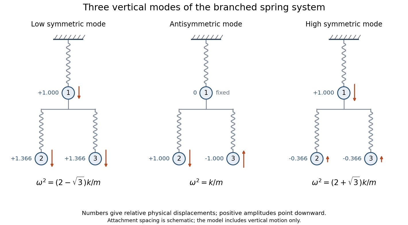
Relative physical climber displacements in the three vertical normal modes; branch spacing is schematic
. Details. 
The left coset isEvery belongs to , because , so the cosets cover . If and intersect, choose in the intersection. Then , so for some . Thus .
Hence two left cosets are either identical or disjoint, and the distinct left cosets form a partition of a set whose union is . Finiteness is unnecessary for this partition argument. In the finite case each coset has members, since multiplication by is a bijection, giving Lagrange's theorem.
Denote a matrix by , with the upper-right entry. Direct matrix multiplication givesThis proves closure. Associativity is inherited from matrix multiplication. The identity is , and the inverse isBoth products with this matrix are the identity. Thus these real matrices form the Heisenberg group, in the coordinate convention with central coordinate .
Let . Its multiplication adds , its identity is and its inverse negates , so it is a subgroup. MoreoverThus every element of is central, and . Therefore is a normal subgroup. In fact it is the full center of a group, as described by the center quotient of the real Heisenberg group.
Perform the product and inverse formulas from part (b) in the commutative ring . They involve only addition, multiplication and negatives, so closure and inverses remain valid; no division by a nonunit is needed. Associativity again comes from matrix multiplication, and remains the identity. The Heisenberg group over a commutative ring therefore hasThese are residues modulo four, not arithmetic in the finite field of four elements.
For the additional subgroup task, write an element of as . Its product and inverse areBoth remain in , and the product is unchanged on exchanging the factors because . The identity is included, so is an Abelian subgroup. There are four independent choices each for , givingThus there are four distinct left cosets. Explicitly the surjective group homomorphism has kernel ; the four cosets are the level sets of that difference, with representatives , . This is the Abelian plane subgroup of the Heisenberg group modulo four.
The kernel of a group homomorphism isThe homomorphism sends identity to identity and inverses to inverses. Thus , and if , then , so is a subgroup by the subgroup test.
For any and ,Hence . Applying the same inclusion with gives equality, provingThis normality argument does not require either group to be finite.
The conjugacy class of isIf is a normal subgroup and , then normality gives for every . Thus the whole conjugacy class of each member of is contained in , andConjugacy classes partition the group, so this is a union of complete disjoint classes, never selected fractions of classes.
The cycle type records the lengths of the disjoint cycles in a permutation, including fixed points as length-one cycles. The possibilities for three objects areThese exhaust the six elements of the symmetric group , denoted in the source. They are also the conjugacy classes of the symmetric group on three letters.
The kernel is a normal subgroup, so it contains the identity class and is a union of the classes listed in part (c). Its candidate orders are therefore , , and . Lagrange's theorem excludes four, since it does not divide six. The remaining possibilities areAll three are normal: the first and last trivially, while is the kernel of the map giving the sign of a permutation, or the index-two subgroup generated by a 3-cycle.
Because is onto, the first isomorphism theorem gives . Explicitly, the map is well defined, multiplicative and surjective; equality of its values means , so it is also injective. ThusEach is realized by the identity map, the sign map and the trivial map, respectively. This completes the classification of normal subgroups and quotients of the symmetric group on three letters.
The table describes the symmetry group of a regular hexagon. Choose as a counterclockwise rotation through and as reflection in one symmetry axis. With , the relations areThe rotation entries already are , and the table gives with indices modulo six. ThereforeThe source writes with the subscript counting polygon vertices; this dihedral group has order 12.
All six reflections square to the identity, and the rotation is the half-turn. These exhaust the nonidentity involutions: has square one only when , giving apart from the identity. Thus the order-two subgroups areA reflection cannot have order three. The rotations of order three are and , and they generate the same subgroup:All these subgroups are cyclic, because a group of prime order is cyclic; the displayed nonidentity elements supply their generators. This gives seven subgroups of order two and one of order three, consistently with involutions in an even dihedral group and the classification of subgroups of a dihedral group.
Act on vectors in the plane of the regular hexagon using its actual rotations and reflections. Choose the first reflection axis as the horizontal axis. A faithful representation is generated byThey are real orthogonal matrices obeying , and . Hence they reproduce the group relations. Since ,This is reflection in the line at angle . More generally . The six rotation matrices are distinct, as are the six reflection matrices; their determinant signs distinguish the two sets. Thus no two group elements have the same matrix, proving faithfulness rather than merely the representation property.
Use the left regular representation, defined on the ordered basis by . Reading the row of the original PDF table gives the permutationThus an explicit permutation matrix, in six-by-six blocks, isEach column has its one in the row labelled by the left product; this specifies the convention completely. Since , the full matrix squares to and is its own inverse. Therefore for every integer, including negative integers,This is also immediate from and the multiplication law for a representation.
The character is the trace. For the planar representation, the rotation trace and reflection trace giveIn the source’s order , these values are .
In the regular representation, the trace counts basis vectors fixed by left multiplication. The equation forces , so a nonidentity element fixes none, while the identity fixes all 12. ConsequentlyIn particular , consistently with the zero diagonal in part (d). The two characters have different identity values because the representation dimensions are two and twelve.
Articles by others on the same topic
There are currently no matching articles.