Options II, Honour School of Mathematics Part A, Trinity Term; Thursday 19 June 2008, 9.30am–12.30pm. The full thirteen-page source, including its intact cover and all nineteen questions, is preserved in a private editable transcription. It was supplied through the past-papers disclosure, in original Part A bundle pages 80–92. Exact departmental worked answers are advertised for H2; that question is retained as an availability record rather than duplicated here. The bounded check found no exact answer advertisement for the other questions.
An invertible matrix is an ordered basis of . After choosing independent columns, their span has elements, so the next column has choices. Thus
For each flag choose an adapted basis: its first vectors span , obtained by extending a basis successively through the nested subspaces and finally through . For two flags, the invertible linear transformation taking one adapted basis to the other takes each member of the first flag to the corresponding member of the second. Hence the action is transitive.
Yes. Suppose maps the first flag to the second and has determinant . Relative to an adapted basis of the first flag, scaling its first basis vector by and fixing all others defines a transformation preserving that flag, with determinant . Then still maps the first flag to the second and has determinant one. Thus the special linear subgroup acts transitively too.
The stabilizer of the indicated flag consists of block upper triangular matrices with diagonal block sizes . The diagonal blocks can be any elements of , and . The upper off-diagonal blocks have arbitrary entries. Thus the stabilizer order is . The orbit-stabilizer theorem gives
The characteristic of a field is the least positive integer with , or zero if none exists. Finiteness forces a positive characteristic, since the sequence of integer multiples of one must repeat. If this least integer factored into two smaller positive factors, their nonzero field multiples would multiply to zero, contradicting the absence of zero divisors. Hence it is prime. The field is a finite-dimensional vector space over its prime subfield , so choosing a basis gives .
A nonzero polynomial of degree over a field has at most roots: each root supplies a linear factor by polynomial division, and induction applies to the quotient. In particular has at most roots. The elements of whose orders divide are precisely those roots. The permitted finite-group criterion therefore proves is cyclic.
For the final assertion take an odd Fermat prime , . Primality forces to be a power of two: an odd factor in would factor nontrivially. Since , the order of two divides but not . As is a power of two, its only divisor not dividing is itself. ThusIt generates the full group exactly when , which holds for and fails for . Therefore the possibilities are , equivalently among odd Fermat primes. The oddness is implicit in referring to two as a unit; is not an admissible case for that claim.
The distinct powers all solve . By the allowed root bound they are all its solutions. A residue of order must therefore equal ; conversely , because characterizes the exponents with . This proves the equivalence with and gives exactly elements of order whenever any such element exists.
To establish existence at the full order too, put and let count elements of order . By Lagrange's theorem for finite groups, these orders divide . The first result gives or . Thereforeusing the standard divisor-sum identity for Euler's function. Equality forces every deficit to vanish, so .
Finally let , which has order eight. Its fourth power is the unique nonidentity square root of one, namely . Since ,because . This proves the stated residue squares to two.
The monotone convergence theorem says that if measurable functions satisfy and converge pointwise to , then is measurable andallowing the common value to be .
No. Take . Each is nonnegative and integrable, and each integral is one. At every fixed real point the functions eventually vanish, so the pointwise limit is zero and its integral is zero. Monotonicity or another convergence hypothesis is essential.
The partial sums are measurable, nonnegative and increasing. By the monotone convergence theorem,A nonnegative measurable function with finite integral is finite almost everywhere: if it were infinite on a positive-measure set, every constant multiple of that set's indicator would be a lower bound, forcing an infinite integral. Thus the series converges almost everywhere.
Substitute , with . The nonnegative integral becomesby scaling and integration by parts. The exponential decays because , with zero boundary term at infinity, proving integrability and
For , the geometric series givesAll terms are nonnegative, so monotone convergence permits termwise integration. Part (i), with , givesThis series is finite for , which also proves integrability of the original nonnegative function.
On a product of sigma-finite measure spaces, Tonelli's theorem equates product and iterated integrals for a nonnegative measurable function, allowing infinite values. Fubini's theorem says that an absolutely integrable measurable function has integrable sections almost everywhere, their section integrals are integrable, and both iterated integrals equal the product integral. Absolute integrability may be checked first by applying Tonelli to the absolute value.
For fixed , Tonelli and the allowed exponential integral giveThe point is irrelevant to the integral. Fubini therefore permits reversing the signed integrals. Evaluating the elementary inner integral yieldsThe first term has integral . The absolute value of the remainder is at mostConsequently the improper integral tends to . The interchange was justified on each finite strip, without asserting absolute integrability on the infinite quadrant.
It is not Lebesgue integrable, because its absolute integral diverges. On , one has and . ThusThese disjoint-interval lower bounds have a divergent harmonic sum. The finite improper value from part (i) is therefore conditional convergence, not Lebesgue integrability.
For a fixed centre , the triangle inequality gives , so the distance-to-centre function is continuous. Its preimage of is the closed ball, hence is closed. Since that closed set contains the corresponding open ball, it contains its closure:Here the bar on the right denotes a closed ball, while the bar on the left denotes closure.
The condition gives the closed squareIts four edges and corners are included, as shown in the left panel of the figure below.
Intersect the ambient balls with . All points on the vertical arm have distance at least from the centre, so the open ball isThe closed ball also contains the endpoints of that segment and the lower half of the vertical arm:The closure of the open ball in is just . Both endpoints are limits of points in the open segment, whereas a vertical point of positive height has a small enough neighbourhood disjoint from it. Thus every point with witnesses strict containment.
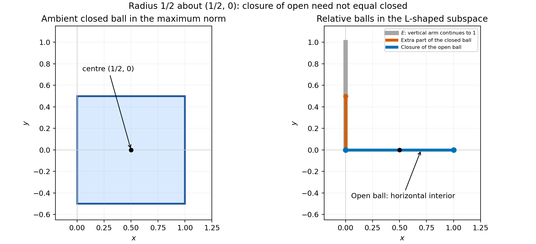
Ambient and relative maximum-norm balls
. The square on the left is the ambient closed ball. On the right, the open ball is the horizontal segment without its endpoints; its closure omits the additional vertical part of the relative closed ball. Details.
Take radius . Part (a) gives one containment. For a point with , define for . Then , while as . Hence every point of the closed ball belongs to the closure of the open ball, proving equality. Positive radius is the standard open-ball convention; a zero-radius open ball would be empty.
In the usual real line, take for . The sets are closed, nonempty and nested, but no real number belongs to all of them.
Every is closed in the Hausdorff ambient space, because it is compact. Inside the compact space , these sets have the finite intersection property: a finite intersection equals the member with largest index and is nonempty. If the total intersection were empty, their open complements would cover ; a finite subcover would contradict that property. Thus
If no were contained in , the sets would be nonempty, nested and compact, since each is closed in . Part (i) would supply a point in , belonging to every but not to , a contradiction. Thus some , and nesting gives the same containment for every later index.
The inclusion holds for every map. Conversely, let belong to the right side. The sets are nonempty and nested. They are compact because singletons are closed in a Hausdorff space and is continuous. By part (b)(i), some lies in every . Then and , proving equality of the two sets.
A two-dimensional embedded submanifold is locally flattened by a continuously differentiable coordinate diffeomorphism of an ambient open neighbourhood onto a coordinate plane, or equivalently locally admits a regular two-parameter chart. A tangent vector at is the velocity of a differentiable curve in through . All such vectors form the two-dimensional tangent space , the image of the differential of a regular parametrization. Normal vectors form its orthogonal complement in , which has dimension one.
The defining function is smooth and has gradient . This cannot vanish on its zero level, since the origin does not lie there. The regular level-set theorem therefore makes a two-dimensional submanifold, with tangent space and normal space
The Lagrange multiplier condition says that at a constrained local extremum of a continuously differentiable objective on a regular surface , its gradient is normal to the tangent plane: for some scalar multiplier.
First the box must be centred at zero. If the two face coordinates in one direction are , subtracting the ellipsoid equations for two vertices differing only in that coordinate gives . A nondegenerate box has , hence . Its positive half-sides therefore satisfy and its volume is .
The feasible closed octant is compact, the boundary gives zero volume, and some interior box has positive volume, so the maximum is interior. Apply multipliers to there:Thus the three squared scaled coordinates are equal and sum to one. The unique positive solution gives
For the regular Sturm-Liouville setting assume is positive and continuously differentiable, are continuous, and . Apply a multiplier to . Its first variation, divided by two, isEndpoint-vanishing variations and the allowed fundamental lemma giveIf an endpoint value is free, its variation is arbitrary, giving the natural condition at that endpoint. At a prescribed endpoint value the variation vanishes there, so no additional natural condition is imposed.
For eigenfunctions with different eigenvalues, multiply their equations by and subtract after integration. The resulting boundary expression vanishes under common homogeneous Dirichlet or common natural boundary conditions. Hence , proving weighted orthogonality.
For the final Dirichlet problem the normalized stationary modes areSolving with both endpoint values zero gives these and excludes nonpositive . Distinct sine modes have zero integral product on . Their Dirichlet values also make the same boundary expression vanish, which explains orthogonality even though their endpoint derivatives do not obey the natural conditions.
For global minimality, the Fourier sine expansion of an endpoint-vanishing function and Parseval's identities give . Equality holds exactly in the first sine eigenspace. ThereforeDistinct modes are orthogonal; the two sign choices of the same minimum are not orthogonal to each other. This distinguishes the family of stationary modes from the two representatives of the minimizing eigenspace in the question's wording.
The Oxford Classical Mechanics revision notice, page 1 explicitly lists AO2 H2 (2008) among the questions with departmental solutions available to Oxford students. Its three source-labelled answer locations are therefore excluded from the original-solution set. The complete source question remains in the private transcription.
The source-free Maxwell equations in vacuum areTheir real and imaginary parts are exactlyPut . Differentiating gives and , while . Thus the necessary and sufficient conditions areHere the complex dot product is bilinear, without complex conjugation. Taking the dot product of the second equation with gives . Crossing it with givesso, since , . Writing , the real conditions areBoth physical fields are linearly polarized: and each oscillate along a fixed real direction. Combining two fields as does not turn the electric field into a circularly polarized field.
The Milne-Thomson circle theorem says that, when is a complex potential analytic inside and on and all its flow singularities are outside, the potential outside an impermeable circle isThe reflected expression is analytic in the exterior: conjugating a local power series turns its argument into . It creates only interior image singularities. On we have , so is real. The stream function is therefore constant on the circle, which is the impermeability condition. At infinity the reflected term is , so it changes the velocity by and leaves the imposed far flow unchanged. These observations prove the theorem, up to the irrelevant additive potential constant and with no extra circulation introduced.
With , , and unit radius, it givesThe image dipole is at with moment ; writing the image term this way changes only an additive constant.
Reflection in the real axis replaces a dipole at with an image at of moment . Reflection in the imaginary axis places the image at with moment . Applying both reflections gives the image at with moment . ThusFor example, on the real axis the first two terms are conjugates and the last two are conjugates. On the imaginary axis the first and third terms are conjugates, as are the second and fourth. The potential is real on each wall, so both walls are streamlines. The only singularity in the open first quadrant is the original dipole.
Reflection in the line is . The printed expression has two conjugation bars: . On the line , this is , which is real; hence its stream function vanishes there. Applying this reflection to the dipole givesConsequentlyThe image lies at , with moment , on the opposite side of the wall.
For each case omit the dipole's own singular field when evaluating the surrounding complex velocity. With the convention this gives , which is the conjugated equation requested in the source. In case (a), differentiating givesFor case (b), differentiate the three image terms:For case (c), differentiation givesThe physical equation for is the complex conjugate of the displayed equation. These expressions apply away from the walls, where the point-dipole model is nonsingular.
Put , and . The circle theorem gives, up to an additive constant,Thus an image source lies at and an image sink at zero. With a counterclockwise contour around the cylinder, Blasius' force theorem isIf locally, the residue of is . The enclosed poles are zero and , with residuesTheir sum is . The residue theorem therefore yieldsThe force points towards the source. For the moment formula the double poles also contribute: . HenceIt follows that andThe zero torque agrees with pressure acting normally to a circle, hence radially through its centre.
The moment generating function is where finite. The continuity theorem states that, if moment generating functions are finite on a common open interval containing zero and converge there to the moment generating function of a probability law, the corresponding distributions converge weakly to that law.
Integrating the gamma density and using the gamma integral givesFor a geometric waiting time, on , summing the geometric series giveswhen . For , deterministically. The waiting times between successive heads are independent and identically distributed, so and . ThereforeIndeed the denominator is and the numerator is . On any sufficiently small fixed neighbourhood of zero these moment generating functions exist for all sufficiently small . The limit is the moment generating function of a gamma law with shape and rate , so
Condition on and apply the Markov property and time homogeneity:Thus the transition matrices satisfy ; since and , induction gives . Averaging over the initial state givesIf , induction gives , so this probability equals for every . This is stationarity of the initial distribution.
A state is recurrent if the probability of returning to at a strictly positive time, starting at , equals one. It is transient if that probability is less than one. If and communicate, choose with and . Chapman-Kolmogorov givesIf is recurrent, summing over makes the right-hand side diverge, so the allowed recurrence criterion proves recurrent. Interchanging proves recurrence is shared throughout a communicating class, and therefore transience is shared too.
For the simple random walk, an odd number of steps cannot return to its starting point, andFor the return series diverges like , proving recurrence. For , , its tail is bounded by a convergent geometric series since , proving transience. At or the walk is deterministic and never returns. Translation invariance transfers the conclusion to every state. Thus recurrence holds exactly when .
Articles were limited to the first 100 out of 126 total.
Articles by others on the same topic
There are currently no matching articles.