Past exam of the physics B course of the University of Cambridge / 2015 / Paper 1 / Section B

In electrostatics, the Maxwell equations in matter areHere ${\rho }_f$ is free charge density and $\mathbf{P}$ is polarization density. For a homogeneous isotropic linear dielectric, the constitutive equation is $\mathbf{D}={ϵ}_0{ϵ}_r\mathbf{E}$. Integrating the first equation over a thin pillbox straddling an interface, with unit normal $\mathbf{n}$ from medium 1 to medium 2, gives $\mathbf{n}\cdot ({\mathbf{D}}_2-{\mathbf{D}}_1)={\sigma }_f$. Integrating the second around a vanishingly narrow rectangular loop gives $\mathbf{n}\times ({\mathbf{E}}_2-{\mathbf{E}}_1)=0$. These are the electrostatic interface boundary conditions. When there is no free surface electric charge, the normal electric displacement field and tangential electric field are continuous; the normal electric field generally is not.

Neglect end fringing field of a capacitor. In either axial segment of the coaxial cylindrical capacitor, a cylindrical Gaussian surface gives $D_r={\lambda }_f/(2\pi r)$, where ${\lambda }_f$ is free electric charge per length. Integrating the radial electric field between the conductors givesThe liquid and air segments share the same conductor electric potential difference, so their capacitances add in parallel. Thus the partially filled coaxial capacitor hasHere the question's $ϵ$ is relative permittivity, and air's relative permittivity is approximated by one.

Write $x$ for the rise above the external level. The wide reservoir keeps that level approximately fixed. At constant applied voltage, one must include work done by the source: the appropriate electrical contribution to the mechanical potential is $-C{V}^2/2$. The upward dielectric insertion force at fixed voltage is consequentlyThe excess hydrostatic pressure $\rho gx$ acts over the annular area $A=\pi (b^2-a^2)$. Alternatively its gravitational potential energy is $\rho gA{x}^2/2$, since liquid initially at the reservoir level must be raised through all heights from zero to $x$. Balancing the derivatives givesThis assumes $h+x<L$, a communicating liquid reservoir, negligible capillarity, and a sufficiently long capacitor that end effects are small. Differentiating gives the dielectric-rise voltmeter's sensitivity at a bias $V$:To obtain its numerical value in $\mu \mathrm{m}{\mathrm{V}}^{-1}$, multiply the right-hand side in SI units by $10^6$. A convenient parametric scale, with $\beta =b/a$, isTODO: a particular numerical sensitivity awaits specified $a,b,\rho ,ϵ$ and operating voltage; none is supplied on the paper. The scale above is a unit-normalized formula, not a claim about the apparatus dimensions or liquid.

The displacement is quadratic in voltage, cannot distinguish its sign, and has zero first-order sensitivity at zero bias. Smaller gaps and larger relative permittivity increase sensitivity, but capillarity, leakage, dielectric breakdown, temperature-dependent liquid properties, and finite available rise then limit performance. A nonconducting liquid avoids a sustained conduction load, although charging still draws electric charge and leakage is possible. A high voltage can give a readable displacement; a low-voltage instrument would require fine displacement measurement and careful calibration.

The differential form of Faraday's law of induction isBy Stokes theorem, for a stationary oriented circuit it becomes $\mathcal{E}=\oint \mathbf{E}\cdot d\mathbf{\ell }=-d{\Phi }_B/dt$, where ${\Phi }_B=\int \mathbf{B}\cdot d\mathbf{S}$ is magnetic flux and $\mathcal{E}$ is electromotive force. Circuit orientation and surface normal obey the right-hand rule. Lenz's law is the physical meaning of the minus sign: the induced current's magnetic field opposes the change in linked magnetic flux. For a moving circuit, the force per unit electric charge is $\mathbf{E}+\mathbf{v}\times \mathbf{B}$, and its line integral is the corresponding electromotive force. Motion through a static magnetic field can therefore induce a voltage even when ${\partial }_t\mathbf{B}=0$.

Let $\theta$ be the wire's angle from the downward vertical, $r=L\sin \theta$, and choose $\mathbf{\omega }$ and $\mathbf{B}$ upward, as in the figure. The motional term along the wire has radial component $B\omega s$ at cylindrical radius $s$. In steady electrical equilibrium, integrating from the grounded axis to the bob givesThe Lorentz force on this positive electric charge is radially outward. Its ratio to the required centripetal term is $QB/(m\omega )\lesssim C{B}^2{L}^2/(2m)$, so the stated heavy-bob condition makes its effect on the zero-field conical pendulum geometry negligible. With wire tension $T_w$, $T_w\cos \theta =mg$ and $T_w\sin \theta =m{\omega }^{2}r$, giving $\cos \theta =g/({\omega }^{2}L)$. Hence the magnetically charged conical pendulum hasA nonzero-radius orbit requires ${\omega }^{2}L>g$. Reversing the sense of rotation or the magnetic field reverses the sign of $Q_0$.

The response to the added electric field requires an electrical convention. In the usual mechanical approximation, treat the pre-existing electric charge as $Q_0$, include its upward electric force $Q_{0}E$, and neglect all magnetic-force feedback. ThenThis predicts an increased radius for $Q_{0}E>0$. It is the result when the newly applied field is used only as a probe force on the original electric charge.

There is a first-order qualification if the bob remains electrically connected to the grounded pivot and the uniform added field's potential is included consistently. Put $s=\cos \theta$ and set the external electric potential to zero at the pivot. The external potential at the bob is then $ELs$, so the charging relation and full force balance becomeThe second equation follows by eliminating the wire tension between vertical balance and radial balance, including the outward magnetic Lorentz force. Expanding both equations to first order in $E$, and to leading order in $C{B}^2{L}^2/m$, with $s_0=g/({\omega }^{2}L)$, givesThe extra factor arises from the added field changing $Q$ by $-CEL{s}_0$ and therefore changing the radial magnetic force. That term is linear in $E$ too; the heavy-bob assumption alone does not justify retaining $Q_{0}E$ while dropping it. The two expressions refer to the two electrical approximations just specified. The expansion requires a small change relative to the initial radius and is nonuniform as that radius tends to zero.

For an electrical measurement, route the grounded connection through a sensitive electrometer operated near zero input voltage, and integrate the charging electric current when $B$ or $\omega$ is changed. Starting with the field off, the transferred electric charge is $Q_0$ in this ideal capacitance model. Reversing $B$ separates the induced signal from offsets. Alternatively, isolate the charged bob briefly and measure its electric potential with a high-input-impedance electrometer, accounting for the instrument's extra capacitance and for the fact that isolation changes the electrical boundary condition.

The characteristic impedance of a lossless transmission line is the ratio of the voltage to the current amplitude of a single forward-travelling wave. If $\mathcal{L}$ and $\mathcal{C}$ denote inductance and capacitance per unit length, the lossless telegrapher equations giveA backward wave has $I_{-}=-V_{-}/Z$ when current is positive along $+z$. Thus characteristic impedance is not a resistor's electrical resistance: it describes travelling-wave amplitudes and determines impedance matching, power transfer and reflections. A semi-infinite line, or a line terminated by a matching load, presents that impedance at its input.

At a junction with no lumped branch, voltage and electric current are continuous:Eliminating $V_t$ gives the voltage reflection coefficientFor real positive $Z_1$, incident and reflected waves occupy the same line, so their power ratio is $|r{|}^2$.

For the slightly mismatched coaxial cables, the change in characteristic impedance isConsequentlyThe requested power limit $0.01\%=10^{-4}$ implies $|\Delta b|/b<0.02\ln (b/a)$. Since $\ln (b/a)=2\pi nZ/Z_{\mathrm{vac}}=1.918$ for the stated line, the adjacent cables' outer radii must match within approximately $3.84\%$. If a tolerance is quoted separately as a symmetric manufacturing range $\pm \delta b$ and arbitrary worst-case pairs can differ by $2\delta b$, the corresponding individual tolerance is approximately $\pm 1.92\%$. The leading calculation is for small mismatches; the exact logarithmic expression gives slightly asymmetric positive and negative limits. The vacuum wave impedance used here is approximately $376.73\Omega$.^[ref]

A needle is a shunt electrical resistance $R_n$, so the load seen at its location is the continuation of the line in parallel with $R_n$: $Z_L=Z{R}_n/(Z+R_n)$. The local voltage reflection coefficient and transmission amplitude areFor periodic resistive loading of a transmission line, the reflection from the next needle travels an additional round trip $2L$ and crosses each previous needle twice. Taking the first needle as phase reference, the single-return approximation for periodic line reflections therefore sums toHere $v_p$ is the propagation phase velocity in the cable, $c/n$ for the stated nondispersive nonmagnetic filling. Squaring the amplitude gives the requested expressionFor a finite number $N$ of needles the amplitude has the additional numerator $1-[t^2{e}^{i\varphi }{]}^N$. The displayed semi-infinite result assumes sufficiently many needles, no terminal reflection, and neglects intrinsic propagation loss.

For real $r<0$, write $q=t^2$. The denominator of the power coefficient is $1+q^2-2q\cos \varphi$. It has constructive peaks at $\varphi =2\pi j$ and minima at $\varphi =(2j+1)\pi$, repeating with frequency spacing $\Delta \nu =v_p/(2L)$. Within this approximation,Weak individual shunts thus give narrow interference peaks, with phase width of order $|r|$.

The requested sum excludes paths that reflect repeatedly between different needles. It should not be read as an exact multiple-scattering result, particularly at the coherent peaks. For example the exact semi-infinite amplitude satisfiesAt $\varphi =2\pi j$ this equation reduces to $(R+1{)}^2=0$: the exact ideal infinite array has unit power reflection there, rather than the first-return approximation's value near $1/4$. This does not change the requested geometric-series derivation, but identifies its physical limitation.

Choose the guide axis as $z$, with $0<x<a$ and $0<y<b$. The electric field is along $y$, parallel to the walls' $b$ dimension. Take a homogeneous lossless nonmagnetic dielectric with relative permittivity $ϵ$, ideal conducting walls, and time dependence $e^{-i\omega t}$. The lowest transverse electric mode of a rectangular waveguide isAt $x=0,a$, this tangential electric field vanishes. At $y=0,b$ the electric field is normal to the wall; a nonzero value is supported by surface electric charge and violates no conducting boundary condition. The field has zero divergence. The associated normal magnetic field also vanishes at each wall, as verified below. The fundamental sine across the wider dimension minimizes the nonzero transverse wave number; ${\mathrm{TE}}_{00}$ is not a physical propagating mode of a hollow simply connected guide.

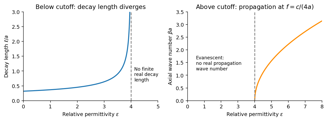
Below the waveguide cutoff frequency $f_c=c/(2a\sqrt{ϵ})$, put $\beta =i\kappa$ with $\kappa >0$ to select decay for $z>0$. The evanescent transverse electric mode in a rectangular waveguide then hasFor the fixed frequency in the question,The decay length increases monotonically and diverges as $ϵ\to 4^{-}$; its formal limit at $ϵ\to 0^{+}$ is $a/\pi$. At $ϵ=4$ the mode is at cutoff, with zero axial wave number. For $ϵ>4$, $\beta =(\pi /a)\sqrt{ϵ/4-1}$ is real and the mode propagates without axial attenuation in this ideal lossless model. There is no real finite evanescent decay length to continue beyond cutoff. The paper's graph notation $l$ denotes the same $\ell$ as its preceding formula.

From Faraday's law of induction, $\nabla \times \tilde{\mathbf{E}}=i\omega \tilde{\mathbf{B}}$. Writing $q=\pi /a$ givesThus $B_x$ vanishes on the $x$ walls and $B_y$ vanishes on the $y$ walls, meeting the normal magnetic boundary conditions. The fields also satisfy $\nabla \cdot \mathbf{B}=0$. For real $E_0$ the physical fields are $E_y=E_0\sin (qx)e^{-\kappa z}\cos \omega t$, $B_x=-(\kappa /\omega )E_0\sin (qx)e^{-\kappa z}\sin \omega t$, and $B_z=-(q/\omega )E_0\cos (qx)e^{-\kappa z}\sin \omega t$.

The time-averaged Poynting vector isAll products are imaginary because the electric field and magnetic field are in quadrature. A single decaying evanescent wave stores reactive energy without transmitting average power into a semi-infinite lossless guide. A finite below-cutoff section can transmit power when both independent evanescent solutions are present; that is a different boundary-value problem.

The skin effect also gives exponential field decay, but in a good metal $k$ has both real and imaginary parts and there is a real inward mean Poynting vector. That flux supplies Joule heating $\sigma |\tilde{E}{|}^2/2$. Here attenuation comes from geometric cutoff in a lossless region, with no conductivity and no dissipative power sink; exponential decay alone does not establish absorption.