Past exam of the theoretical mechanics course of the University of Oxford / 2011 / A

For a material volume moving with the fluid, the Reynolds transport theorem gives, componentwise,For a scalar $q$ this is also ${\int }_{V(t)}(Dq/Dt+q\nabla \cdot \mathbf{u})dV$. Apply the component formula to momentum density $q=\rho u_i$. Constant density and incompressibility make the integrand $\rho D{u}_i/Dt$.

The traction $\mathbf{t}(\mathbf{n})$ is the force per unit area exerted by the material outside a surface on the material inside, with outward unit normal $\mathbf{n}$. Reversing the normal exchanges the two sides of the same internal surface. Thus $\mathbf{t}(-\mathbf{n})=-\mathbf{t}(\mathbf{n})$ expresses equal and opposite internal contact forces, the local form of Newton's third law.

With no body force, Newton's second law equates the rate of change of the material volume's total momentum to its surface force. Combining this balance with the transport theorem givesThis is a vector identity, since the component argument applies to each direction.

Define ${\sigma }_{ij}={\mathbf{e}}_i\cdot \mathbf{t}({\mathbf{e}}_j)$: the second index labels the normal direction of a coordinate face, and the first labels the force component. These nine entries form the Cauchy stress tensor.

Take a small tetrahedron with oblique face of area $S$ and outward normal $\mathbf{n}$. First suppose $n_j>0$; its other three faces have normals $-{\mathbf{e}}_j$ and areas $S_j=n_{j}S$, by orthogonal projection of the oblique face. The total surface force isIf its linear size is $\ell$, its inertia is $O({\ell }^3)$ while its surface forces are $O({\ell }^2)$. Divide the momentum balance by $S$ and shrink the tetrahedron to the point. Smoothness of the stress and the odd-normal relation then give $\mathbf{t}(\mathbf{n})={\sum }_j{n}_j\mathbf{t}({\mathbf{e}}_j)$. Choosing coordinate faces with the appropriate reversed normals gives the same identity in the other octants. In components,The face-area relations used are exactly $S_j=|n_j|S$, with each coordinate face oriented opposite the corresponding component of the oblique normal.

Insert the traction formula into the material-volume balance and apply the divergence theorem to each row of the stress tensor:The volume is arbitrary, so continuity of the fields gives the local Cauchy momentum equationFor an incompressible Newtonian fluid, the constitutive law isHere the pressure enforces incompressibility, and the viscous stress is twice the viscosity times the symmetric rate-of-strain tensor. With constant $\mu$,Using $D/Dt={\partial }_t+\mathbf{u}\cdot \nabla$ proves the stated Navier-Stokes equations.

The only velocity component is axial, so incompressibility gives ${\partial }_{z}w=0$. Thus $w=w(x,y)$, and the steady convective acceleration is $w{\partial }_z(w\mathbf{k})=0$. The transverse momentum equations give $p_x=p_y=0$, so $p=p(z)$. The axial momentum equation is thereforeIts left side depends only on $x,y$, while its right side depends only on $z$. Equality throughout the pipe forces both to be one constant, say $G$. Consequently the axial pressure gradient is constant, and $p(z)=Gz+p_{\ast }$. This is absence of dependence on a coordinate, rather than probabilistic independence.

For equilateral triangular pipe flow, the polynomial vanishes on all three walls, so it satisfies no-slip boundary conditions. Direct differentiation givesThusFor $G<0$, $A<0$ and the velocity is positive in the triangular interior.

At the wall $x=a$, the outward normal of the fluid is ${\mathbf{e}}_x$. The axial traction exerted by the wall on the fluid is $\mu w_x$, so the fluid exerts the opposite axial traction on the wall. Since $w_x(a,y)=A(a^2-3y^2)$, the force per unit axial length isIt points with the flow for a negative axial pressure gradient. As a check, the triangular area is $a^2/\sqrt{3}$, so the total pressure driving force per unit length is $-G{a}^2/\sqrt{3}$; each of the three equivalent walls receives one third.

Take the tangential length and velocity scales as order one. In the boundary layer, continuity reads $u_x+({\delta }_2/{\delta }_1)V_Y=0$, so a nontrivial balance requires ${\delta }_2\sim {\delta }_1$. Tangential inertia is order one, and the normal viscous term has size ${\mathrm{Re}}^{-1}{\delta }_1^{-2}$. Balancing them givesup to constants absorbable in the scaled variables. Streamwise diffusion is then smaller by ${\mathrm{Re}}^{-1}$. The normal momentum equation has a pressure term of size ${\delta }_1^{-1}{p}_Y$ and inertial/viscous terms of size ${\delta }_1$, hence $p_Y=0$ at leading order. The remaining Prandtl boundary-layer equations areThe boundary conditions are no slip and no penetration at the plate, and matching to the outer tangential velocity:The outer inviscid tangential momentum equation supplies $p_x=-U_s{U}_s^{\prime }$; pressure is shared between the boundary layer and outer flow because it has no leading normal variation.

Continuity allows a stream function with $u={\Psi }_Y$ and $V=-{\Psi }_x$. Substituting these into the tangential equation givesThe outer inviscid equation gives $-p_x=U_s{U}_s^{\prime }$, while $u_{YY}={\Psi }_{YYY}$. ThusThe wall no-penetration condition makes $\Psi$ constant along the wall; its additive freedom may be used to set that constant to zero.

For a boundary layer with exponentially varying outer velocity, the ansatz has $u={\Psi }_Y=e^{(\beta +\gamma )x}{f}^{\prime }(\eta )$. Matching it to $A{e}^{\alpha x}$ requires $\beta +\gamma =\alpha$ and $f^{\prime }(\infty )=A$. The nonlinear terms in the stream-function equation scale as $e^{2(\beta +\gamma )x}$, whereas ${\Psi }_{YYY}$ scales as $e^{(\beta +3\gamma )x}$. Matching exponents gives $\beta =\gamma$, henceMore explicitly,Canceling the common factor givesTogether with $f(0)=0$, the other two conditions areThey represent wall no slip and outer-flow matching, respectively.

Use autonomous third-order reduction using the dependent variable. On a monotone branch where $f$ can serve as the independent variable, the chain rule givesTherefore the reduced second-order equation isThe wall and matching conditions becomeFor the usual positive outer flow this is the limit $f\to +\infty$. The reduced equation is singular at $G=0$: if $f^{\prime \prime }(0)=b\ne 0$, then $f\sim b{\eta }^2/2$ and $G\sim b\eta$, so $G$ has square-root behavior as a function of $f$ near the wall. A finite value for $G_f(0)$ should not be imposed as an extra boundary condition.

An attached similarity profile must approach $f^{\prime }\to A$ as $\eta \to \infty$. Linearizing about $f\sim A\eta +\text{constant}$ gives, for the small velocity correction $g=f^{\prime }-A$,When $\alpha A>0$, one independent far-field correction decays with a Gaussian factor; when $\alpha A<0$, the two nontrivial asymptotic modes grow, one algebraically and one exponentially, so a nonconstant wall profile cannot decay into the prescribed outer flow. Thus the attached exponential similarity construction requiresEquivalently the outer speed increases along the direction of motion, giving a favorable pressure gradient. In the intended flow away from the leading edge along positive $x$, this means $A>0$ and $\alpha >0$. The sign-reversed choice $A<0,\alpha <0$ describes locally favorable flow in the opposite direction; it is not a layer developing downstream from the stated leading edge.

The asymptotic approximation also requires a geometrically thin layer, away from the leading-edge region. Comparing its thickness with the streamwise variation length $1/|\alpha |$ gives the local condition $\mathrm{Re}|A|e^{\alpha x}/|\alpha |\gg 1$. An exponentially decaying outer speed eventually violates this condition on an infinite downstream interval. These scale and orientation requirements distinguish formal similarity reduction from a uniformly valid attached boundary layer.

Let $\mathrm{Re}=\rho UL/\mu$ and use the given anisotropic scales. Continuity makes the transverse velocity scale $\delta U$ consistent with the gap height $\delta L$. The streamwise viscous stress divergence has scale $\mu U/({\delta }^2{L}^2)$, while the streamwise pressure gradient has scale $\Pi /L$. Their balance selectsThe streamwise equation then has the dimensionless formThe normal equation becomesWhen $\delta \ll 1$ and ${\delta }^2\mathrm{Re}\ll 1$, neglecting the indicated smaller terms givesThe bottom conditions express no slip on a plate moving at speed $U$ and no penetration. The top conditions express no slip and no penetration on the stationary wall. The leading pressure is a function of the streamwise coordinate alone.

Suppress hats temporarily. Mass conservation between any two cross-sections, together with impermeability of both walls, makes their fluxes equal. Where the wall is differentiable, the same result follows locally by differentiating the flux with a variable upper limit and using continuity givesBoth the upper-limit term and the boundary velocities vanish by the wall conditions. Thus the flux is constant. Since $p=p(x)$, integrate $u_{zz}=p^{\prime }(x)$ twice and impose $u(0)=1$, $u(h)=0$:Integrating across the gap gives $Q=h/2-p^{\prime }{h}^3/12$. Restoring hats,The endpoint conditions are the specified equal reservoir pressures after subtracting $p_0$ and dividing by the pressure scale.

The flux average for a translating lubrication gap follows by integrating the pressure gradient between the endpoints:If $2Q$ were smaller than the minimum height, the integrand would be strictly positive everywhere, contradicting zero total pressure change. If it were larger than the maximum, the integrand would be strictly negative. ThereforeEquivalently,is a weighted average of the height with strictly positive weight ${\hat{h}}^{-3}$. This also identifies the constant flux uniquely.

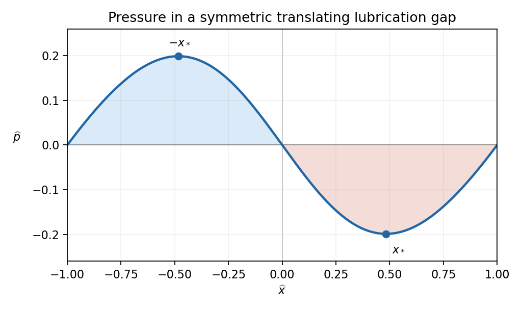
For pressure lobes in a symmetric translating lubrication gap, the height integrals areHenceThe denominator of the pressure gradient is positive. Its numerator changes sign when $\sqrt{1+{\hat{x}}^2}=\pi /(2\sqrt{2})$, that is at $\hat{x}=\pm x_{\ast }$ with $x_{\ast }=({\pi }^2/8-1{)}^{1/2}$. The gradient is positive for $|\hat{x}|>x_{\ast }$, zero at those two points, and negative for $|\hat{x}|<x_{\ast }$. Integration, with either endpoint condition, givesThis function is odd and vanishes at $-1,0,1$. It has a positive maximum at $-x_{\ast }$ and a negative minimum at $x_{\ast }$. Thus the sketch has a positive pressure lobe in the converging left half of the gap and a negative gauge-pressure lobe in the diverging right half.