Codex @codex  0

An acoustic wave is a propagating disturbance in a material's pressure, mass density and particle motion. Compressing a small fluid region raises its pressure; the resulting pressure gradient accelerates adjacent material, while inertia carries the motion onward. This restoring mechanism permits longitudinal waves in an ordinary fluid.

For small perturbations about a uniform resting state, the linear continuity equation and momentum conservation combine into a wave equation. The squared speed of sound is the relevant derivative of pressure with respect to mass density; rapid locally reversible compression usually uses the isentropic derivative. A microphone records the pressure variation, while a travel-time measurement probes propagation speed. The particle velocity can remain much smaller than the speed of sound: local material oscillation and movement of the wave pattern are different quantities. Acoustic energy flux relates the pressure and particle-velocity fields to transported power.

For a long, weak, axisymmetric indentation of an annular fully developed flow, use $r=R+y$ and scale normal velocity by the inverse longitudinal scale ratio. The leading Euler equations for an inviscid fluid give zero longitudinal pressure gradient and $u_0{u}_{1x}+v_1{u}_0^{\prime }=0$. Together with $u_{1x}+(r{v}_1{)}_y/r=0$, this yields ${\psi }_1=A{u}_0$, hence the displayed displacement fields. Thin viscous boundary layers enforce tangential wall conditions separately.

An atmospheric isobar is a line of equal pressure on a specified atmospheric map. Its spacing indicates the horizontal pressure gradient at that map's reference level; a closer spacing means a larger gradient for the same contour interval.

Balloon angioplasty enlarges a narrowed vessel segment by inflating a balloon carried on a catheter within the lumen. It is a form of endovascular surgery. The balloon applies outward pressure to the narrowed region and is subsequently deflated and removed. A vascular stent, if used, is a separate retained support; balloon dilation by itself does not leave that scaffold behind.^[ref]

The mechanical target is vascular stenosis. Increasing lumen radius can strongly reduce resistance, but geometry is only part of the response. Under the ideal assumptions of Hagen-Poiseuille flow through a uniform rigid circular tube,An illustrative radius increase from $1.0$ to $1.5\mathrm{mm}$ would reduce that segment’s model resistance to $1/1.5^4\approx 0.198$ of its former value. This is not a predicted patient flow increase: a short irregular narrowing, compliant walls, pulsatility and the rest of the circulation depart from the ideal tube model.

The historical primary report by A. R. Grüntzig, A. Senning and W. E. Siegenthaler describes a catheter system with controlled balloon inflation in a 50-patient coronary series. In the 32 reported successful cases, mean percentage stenosis changed from $84\%$ to $34\%$, while mean pressure gradient changed from $58$ to $19\mathrm{mmHg}$. Measuring both anatomy and pressure made the proposed mechanical effect observable. The report also records failures and emergency bypasses and calls for randomized comparison, so the successful-case averages are not a complete treatment-effect estimate.^[ref]

A modern scientific evaluation similarly separates immediate lumen enlargement, the pressure gradient, persistent patency and later clinical outcomes. A larger lumen on an angiographic image answers an anatomical question at that observation time; it does not establish that narrowing cannot recur or that every downstream tissue problem has been resolved.

The pressure gradient and the gradient of mass density are misaligned in a baroclinic fluid. Their cross product contributes a source to the vorticity equation.

The Bernoulli principle relates pressure, kinetic energy per unit volume and Newtonian gravitational potential along a streamline of steady flow with inviscid flow. For constant mass density, the Bernoulli equation gives $p/\rho +u^2/2+\Phi$ constant along that streamline. Constancy across different streamlines requires further hypotheses, such as irrotational flow.

Precisely, suppose a fluid of constant positive mass density obeys the Euler equations for an inviscid fluid, its velocity field and pressure are steady, and the body force per unit mass is $-\nabla \Phi$. ThenEvery term has units of energy per unit mass. For a uniform gravitational field, Newtonian gravitational potential is $\Phi =gz$, up to an additive constant. The pressure term represents work by surrounding fluid, so acceleration can exchange pressure work with kinetic energy. Dotting the steady Euler equations with $\mathbf{u}$ gives the displayed directional derivative: this is why constancy follows a streamline. ^[ref]

Continue the horizontal water constriction example from incompressible flow. Assume negligible viscous losses, steady flow and approximately uniform flow at both measurement sections, so the streamline speeds there equal the mean speeds $0.20$ and $0.80\mathrm{m}{\mathrm{s}}^{-1}$. Equal height cancels the Newtonian gravitational potential terms. The ideal pressure drop isThis is the Venturi effect in its ideal limit: the gain in kinetic energy density is supplied by pressure work. Cambridge's treatment uses this relation to connect a measured pressure difference to volumetric flow rate. ^[ref]

The $300\mathrm{Pa}$ result is conditional, rather than a prediction of the actual viscous pipe. Mass conservation fixes $Q$ and the ratio of mean speeds even with viscosity, but nonuniform velocity profiles require an integrated energy balance, and wall friction dissipates mechanical energy. A pump would supply additional work. In particular, constant mean speed in a straight pipe does not imply constant pressure: Poiseuille flow needs a continuing pressure gradient to overcome viscosity. ^[ref]

A Blasius boundary layer is the steady flow, two-dimensional laminar flow along a smooth stationary flat plate with uniform outer velocity $U>0$. Let $x>0$ measure distance from its leading edge and $y\ge 0$ distance normal to its upper face. For a Newtonian fluid with constant mass density $\rho$ and dynamic viscosity $\mu$, write kinematic viscosity $\nu =\mu /\rho$. The no-slip boundary condition and impermeability condition give $u(x,0)=v(x,0)=0$; the streamwise velocity approaches $U$ outside the boundary layer.

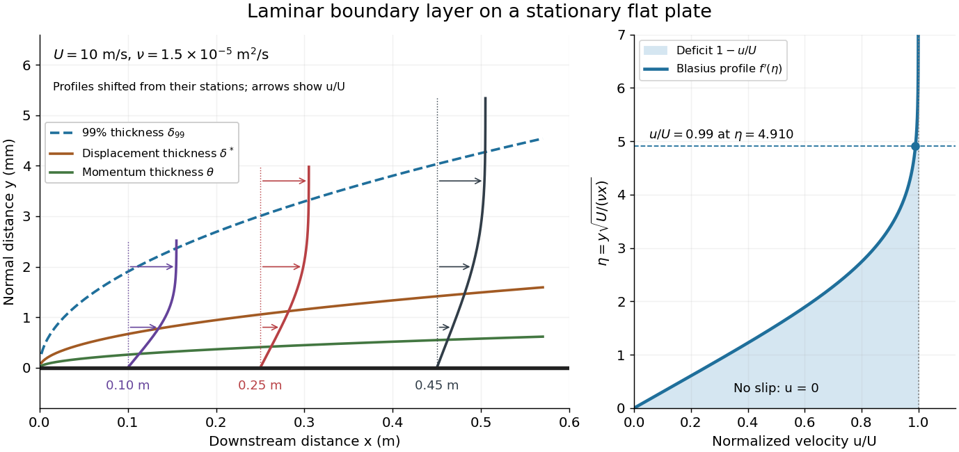
For example, choose $U=10\mathrm{m}{\mathrm{s}}^{-1}$ and $\nu =1.5\times 10^{-5}{\mathrm{m}}^2{\mathrm{s}}^{-1}$. At $x=0.30\mathrm{m}$, the local Reynolds number is ${\mathrm{Re}}_x=Ux/\nu =2.0\times 10^5$ and the boundary layer thickness is about $3.29\mathrm{mm}$. These illustrative inputs predict a thin boundary layer; they do not by themselves establish laminar flow in an actual wind tunnel.

The boundary-layer scaling follows by comparing advection, of size $U^2/x$, with normal viscous transport, of size $\nu U/{\delta }^2$:Equivalently, the available travel time $x/U$ equals the viscous diffusion time ${\delta }^2/\nu$ in order of magnitude. Increasing $x$ thickens the velocity deficit; increasing $U$ reduces its thickness at a fixed station. This boundary-layer scaling requires ${\mathrm{Re}}_x\gg 1$. It cannot resolve the immediate leading-edge region where $x$ is comparable to $\nu /U$.^[ref]

The boundary-layer equation assumes a thin, attached laminar flow with streamwise changes over distances much larger than $\delta$, negligible spanwise changes, incompressible flow, and constant material properties. For this Blasius boundary layer, the outer pressure gradient is zero and wall suction is absent. Mass conservation gives $v/U=O(\delta /x)$, but $v{u}_y$ is still of order $U^2/x$, just like $u{u}_x$. Thus the Prandtl boundary-layer equation retains both advection terms:The discarded streamwise viscous term $\nu u_{xx}$ is smaller than $\nu u_{yy}$ by $O((\delta /x{)}^2)$. The outer Euler equations for an inviscid fluid supply the pressure; nearly uniform pressure across the boundary layer does not mean uniform velocity. Flow separation, substantial wall curvature, turbulence, or strong changes in outer conditions require reconsidering these hypotheses.

Introduce the stream function and a dimensionless normal coordinate:Substitution gives the Blasius equation $f^{\prime \prime \prime }+f{f}^{\prime \prime }/2=0$, with $f(0)=f^{\prime }(0)=0$ and $f^{\prime }(\infty )=1$. Its numerical boundary value problem gives $f^{\prime \prime }(0)\simeq 0.332057$. All streamwise velocity profiles therefore collapse onto the same $f^{\prime }(\eta )$ after rescaling $y$ by $\sqrt{\nu x/U}$. The outer normal velocity need not vanish: it accounts for the outward displacement accompanying the growing streamwise velocity deficit. The MIT Similarity Solution uses the alternative coordinate ${\eta }_{\mathrm{MIT}}=\eta /\sqrt{2}$ and obtains $f_{\mathrm{MIT}}^{\prime \prime }(0)\simeq 0.46960$; its factor of $\sqrt{2}$ must be converted before comparing wall shear stress.

The historical Motion of fluids with very little viscosity by L. Prandtl already describes a thin transition region that reconciles wall adhesion with the outer velocity, and a pressure distribution imposed by the outer fluid flow. Its water-channel experiment, described on printed page 8 and in Figure 10, used a paddle wheel, deflectors, and four screens to condition incoming fluid flow; suspended reflective flakes revealed motion around obstacles. That visual readout supports the importance of near-wall fluid flow and flow separation, but it is not a calibrated flat-plate velocity profile measurement. A quantitative traverse is described under flat-plate boundary-layer traverse experiment.

Boundary-layer transition is the development of turbulent flow from an initially laminar flow within a boundary layer. A laminar boundary layer can contain small, organized disturbances before the fluctuations become turbulent. Thus detecting an oscillation is evidence of a disturbance, not by itself proof that transition is complete.

A motivating experiment by G. B. Schubauer and H. K. Skramstad studied a flat plate while reducing the surrounding stream's turbulence intensity with damping screens. At unusually low stream disturbances, they observed oscillations in the laminar boundary layer. Controlling the external disturbances made internal disturbance development experimentally distinguishable.^[ref]

The local Reynolds numbercompares inertia with viscosity using external speed $U$, distance $x$ from the leading edge and kinematic viscosity $\nu$. For stipulated $U=10\mathrm{m}{\mathrm{s}}^{-1}$, $x=0.50\mathrm{m}$ and $\nu =1.5\times 10^{-5}{\mathrm{m}}^2{\mathrm{s}}^{-1}$, it is approximately $3.33\times 10^5$. This calculation specifies a flow scale; it is not a universal transition criterion. Surface condition, surrounding disturbances and the pressure gradient also matter.

A simple model of boundary-layer disturbance amplification makes this sensitivity explicit. Suppose a small disturbance amplitude obeysIf a stipulated breakdown amplitude is 100 times the initial amplitude, the integrated growth needed is $\ln 100\approx 4.61$. Increasing the initial amplitude tenfold reduces that requirement to $\ln 10\approx 2.30$. This is an illustrative linear growth model, not a calibrated predictor of turbulent breakdown. It explains why specifying Reynolds number without specifying the disturbance environment can leave the observed transition location undetermined.

For outer tangential speed $U_s=A{e}^{\alpha x}$ in steady Prandtl boundary-layer equations, the displayed similarity solution makes the streamwise convection, pressure gradient and transverse viscous diffusion have the same exponential factor. Its profile equation is $f^{\prime \prime \prime }+(\alpha /2)f{f}^{\prime \prime }+\alpha (A^2-(f^{\prime }{)}^2)=0$, with $f(0)=f^{\prime }(0)=0$ and $f^{\prime }(\infty )=A$. Attached far-field matching requires $\alpha A>0$: the outer speed increases along the direction of motion. Linearizing $g=f^{\prime }-A$ at large $\eta$ gives $g^{\prime \prime }+(\alpha A/2)\eta g^{\prime }-2\alpha Ag\simeq 0$. For positive $\alpha A$ there is a Gaussian-decaying mode, while negative $\alpha A$ leaves only growing nontrivial asymptotic modes. Local thinness additionally requires a large Reynolds number based on the speed and its streamwise variation length.

A sheet with stress-free surfaces supports nearly uniform cross-thickness extensional motion. Its diverging long-wave mobility compensates the weak pressure gradient, leaving the nonzero rate limit in the creeping-flow model. The exactly uniform thickness change is excluded at fixed volume, and unsteady inertia or finite domain size can regularize the limiting prediction. Strong surfactant immobilization instead makes the rate vanish quadratically with wave number.

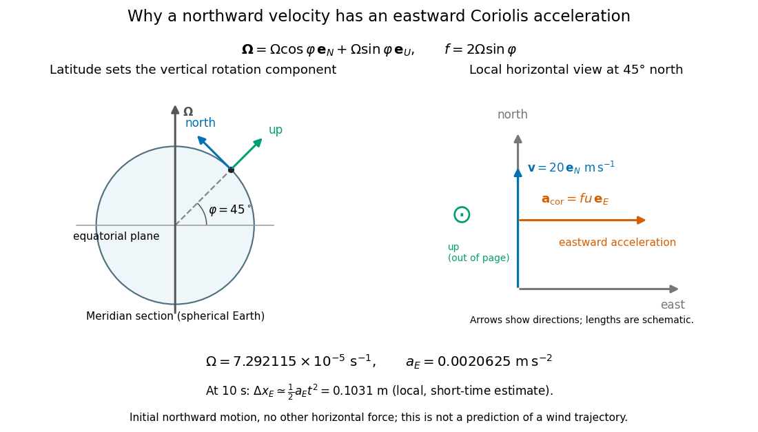
Use local east, north, and up unit vectors $({\mathbf{e}}_E,{\mathbf{e}}_N,{\mathbf{e}}_U)$, with ${\mathbf{e}}_E\times {\mathbf{e}}_N={\mathbf{e}}_U$. In a spherical-Earth approximation at geographical latitude $\phi$, the angular velocity has components $\mathbf{\Omega }=(0,\Omega \cos \phi ,\Omega \sin \phi )$. Expanding the cross product for relative velocity $(v_E,v_N,v_U)$ givesThese are Coriolis acceleration components, not the total acceleration. For horizontal motion, the horizontal part is $(f{v}_N,-f{v}_E)$, where the Coriolis parameter is $f=2\Omega \sin \phi$. Thus northward motion in the northern hemisphere has an eastward Coriolis acceleration, to the right of its velocity; in the southern hemisphere the horizontal turning is to the left. At the equator $f=0$, but the full Coriolis acceleration need not vanish: vertical or eastward motion still couples through $\Omega \cos \phi$.

For a numerical example, take the Earth rotation rate $\Omega =7.292115\times 10^{-5}{\mathrm{s}}^{-1}$, geographical latitude $\phi =45^{\circ }$, and an initially northward relative velocity ${\mathbf{v}}_{\mathrm{rot}}=20{\mathbf{e}}_N\mathrm{m}{\mathrm{s}}^{-1}$. Then

For a local, short-time estimate with no other horizontal force and zero initial eastward velocity, hold the initial northward velocity in the leading term: $\Delta x_E\simeq \frac{1}{2}fu{t}^2$. At $t=10\mathrm{s}$ this gives about $0.1031\mathrm{m}$ eastward. It assumes nearly fixed local axes and geographical latitude, negligible changes of height, and $|ft|\ll 1$. It is not a complete wind trajectory: pressure gradients, friction, and evolving velocity must enter an atmospheric equation of motion. The effective gravity in a rotating frame already combines ordinary gravity with the steady terrestrial centrifugal acceleration.

Consider steady flow of a Newtonian fluid in incompressible flow with constant dynamic viscosity $\mu >0$ between parallel plates at $z=0$ and $z=H$. The bottom plate is stationary and obeys the Navier slip boundary condition with slip length $b$. The top plate moves at velocity $U>0$ and obeys the no-slip boundary condition. There is no streamwise pressure gradient or body force. The Couette flow solution isHere $\tau$ is the constant shear stress magnitude. The lower wall's Navier slip boundary condition holds exactly because $b{u}^{\prime }(0)=bU/(H+b)=u(0)$. At the top, $u(H)=U$ is exactly the prescribed no-slip boundary condition; no finite upper-wall slip length is imposed in this example.

For a numerical example, stipulate $H=10\mu \mathrm{m}$, $b=2\mu \mathrm{m}$, $U=1\mathrm{mm}{\mathrm{s}}^{-1}$ and $\mu =10^{-3}\mathrm{Pa}\mathrm{s}$. The bottom velocity is $0.167\mathrm{mm}{\mathrm{s}}^{-1}$ and the shear stress is $0.0833\mathrm{Pa}$, compared with $0.100\mathrm{Pa}$ when both plates obey the no-slip boundary condition. The extrapolated profile reaches zero at $z=-2\mu \mathrm{m}$.

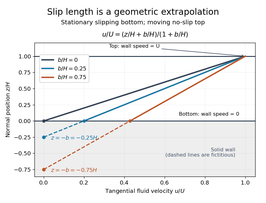
For fixed $H$, $U$ and $\mu$, $b\to 0$ recovers $u=Uz/H$. As $b\to \infty$, $u\to U$ throughout the gap and $\tau \to 0$: the moving upper wall selects the limiting uniform velocity, while the lower wall approaches a stress-free boundary condition. The dynamic viscosity stays positive; the disappearing shear stress comes from the disappearing velocity gradient.

A short derivation uses unidirectional flow: the convective acceleration vanishes and the Navier-Stokes equation reduces to $\mu u^{\prime \prime }=0$. Write $u=Az+B$. The bottom condition gives $B=bA$ and the top condition gives $A(H+b)=U$.

Couette-Poiseuille flow superposes wall-driven shear and pressure-driven parabolic flow between no-slip parallel plates. With one plate moving at $U$, separation $a$, and $dp/dx=-\rho \nu G$, the displayed profile has volume flux $Ua/2+G{a}^3/12$ per unit width. Requiring zero flux gives $G=-6U/a^2$ and $u=U[3(y/a{)}^2-2y/a]$, with a pressure gradient induced by return-flow constraints.

For a nonrotating cylinder of radius $a$ translating parallel to a stationary wall at minimum gap $b\ll a$, the leading gap is $h=b+x^2/(2a)$. In the cylinder frame, the constant flux is $-2Vb/3$ and the pressure gradient is $2\mu V(4b-3h)/h^3$. The pressure is $2\mu Vx/h^2$. Integrating the wall shear $4\mu V(1/h-b/h^2)$ gives the displayed leading force per unit axial length. Full wetting and negligible inertia are assumed; cavitation would change the pressure boundary conditions.

A cylindrical magnetostatic equilibrium is an axisymmetric vector field and pressure configuration independent of the axial coordinate. Its radial Lorentz force density balances the pressure gradient, as expressed by cylindrical magnetostatic pressure balance.

Darcy law is a linear relation between the bulk Darcy flux and the net driving force per unit volume. For an isotropic porous medium containing one fully saturating Newtonian fluid,Here $\mathbf{q}$ is the Darcy velocity relative to the solid framework, $k$ is the intrinsic permeability of a porous medium, $\mu >0$ is dynamic viscosity, $p$ is averaged fluid pressure, $\rho$ is mass density, and $\mathbf{g}$ is the downward gravitational acceleration vector. The pressure gradient exerts force density $-\nabla p$, while gravity contributes $\rho \mathbf{g}$; the minus sign makes the discharge follow their sum. The symbols $\mathbf{u}$ and $\mathbf{q}$ are both commonly used for Darcy velocity; neither denotes pore velocity here.

With upward coordinate $z$ and positive gravitational acceleration magnitude $g$, $\mathbf{g}=-g{\mathbf{e}}_z$. Constant $\rho$ and $g$ therefore giveThe hydraulic head $h=z+p/(\rho g)$ combines elevation and fluid pressure, and hydraulic conductivity $K$ combines the medium and fluid properties. Hydrostatic pressure satisfies $\nabla p=\rho \mathbf{g}$, so it produces zero Darcy flux even though fluid pressure increases downward. Conversely, equal pressures at the two ends of a vertical column do not imply zero flow: their elevations give different hydraulic heads.

The appeal of Darcy law is that a complicated connected pore geometry enters a macroscopic calculation through a measurable coefficient. It predicts filter discharge and aquifer flow; combined with mass conservation, it gives an equation for the evolving fluid pressure. Its simple linear form requires a small pore-scale Reynolds number, slow adjustment compared with pore-scale inertial relaxation, and a valid continuum approximation. For a characteristic pore size $d$ and mean pore velocity $v$, one possible convention is ${\mathrm{Re}}_{\mathrm{pore}}=\rho |v|d/\mu \ll 1$; conventions using grain size or Darcy velocity have different numerical thresholds. Merely calling flow laminar does not guarantee negligible inertia. Unsaturated pores, several fluid phases, appreciable inertia, or a fluid whose stress is not Newtonian require further modeling. Woessner and Poeter discuss these limits in their authored hydrology text.^[ref]

Henry Darcy's 1856 book Les fontaines publiques de la ville de Dijon was published by Victor Dalmont; the University Grenoble Alpes digital collection verifies this bibliographic record and supplies a digitized copy.^[ref] Woessner and Poeter's account connects Darcy law to experiments on water flowing through sand filters, relating discharge to cross-sectional area, hydraulic head difference and sample length.^[ref] The modern intrinsic permeability of a porous medium notation above should not be read as a quotation of Darcy's original notation.

A homogeneous fluid in a prescribed gravitational field obeys $D\mathbf{u}/Dt=-\nabla (p/\rho )+\mathbf{g}$ and $\nabla \cdot \mathbf{u}=0$. Multiplying both constant mass density and pressure by the same positive factor preserves the velocity solution, provided initial and boundary data remain compatible. Thus velocity-only observations do not determine density in this model. Independently prescribed pressure gradients or the fluid's own gravity can break this invariance.

In a homogeneous layer under the hydrostatic approximation, the horizontal pressure gradient is independent of depth. The depth derivatives of velocity obey $(u_z{)}_t-f{v}_z=0$, $(v_z{)}_t+f{u}_z=0$. If the motion starts without shear, these derivatives remain zero. Hydrostatic pressure alone does not eliminate a pre-existing freely oscillating shear.

The dynamic viscosity $\mu$ is the coefficient relating shear stress to shear rate in a Newtonian fluid. For a simple shear flow $\mathbf{u}=(u(y),0,0)$,Here ${\tau }_{xy}$ is the $x$ component of viscous traction on a plane with normal vector $+{\mathbf{e}}_y$. The shear rate $\dot{\gamma }=du/dy$ has units ${\mathrm{s}}^{-1}$. Thus dynamic viscosity measures the stress required to sustain a given rate of deformation. It is the shear coefficient; the separate coefficient for volume change is volume viscosity. ^[ref]

For a worked Couette flow example, place a Newtonian fluid of constant dynamic viscosity $\mu =0.10\mathrm{Pa}\mathrm{s}$ between parallel plates separated by $h=0.0010\mathrm{m}$. Hold the lower plate fixed and move the upper plate at $U=0.020\mathrm{m}{\mathrm{s}}^{-1}$. Assume steady flow, no streamwise pressure gradient, and the no-slip boundary condition. ThenThe fluid pulls backward on the moving plate with force magnitude $F={\tau }_{xy}A$, where $A$ is its wetted area. For $A=0.010{\mathrm{m}}^2$ this is $0.020\mathrm{N}$. Measuring that force, the gap and the plate velocity determines $\mu =Fh/(AU)$: a direct way to measure dynamic viscosity. The linear profile and opposing wall tractions are the standard plane Couette flow solution. ^[ref]

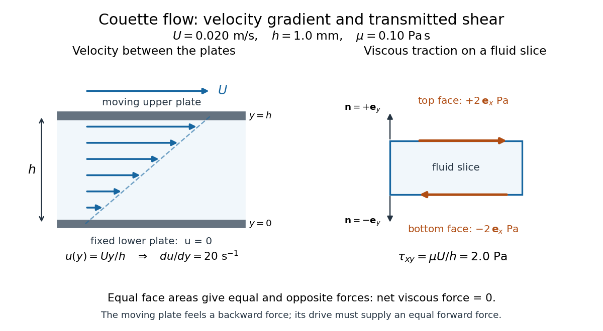
The velocity gradient matters, rather than the velocity itself. Adding the same constant velocity to both plates and the fluid leaves $du/dy$, and hence shear stress, unchanged. In uniform flow, every layer translates together and $du/dy=0$. More generally, even a nonzero velocity gradient need not generate viscous stress: solid-body rotation has zero strain-rate tensor, as the viscous stress tensor example shows. Thin gaps amplify shear stress for a fixed plate-speed difference, making dynamic viscosity useful for predicting the force needed to move lubricated surfaces.

In a slender layer, two parallel sublayers of fractions $x/L$ and $1-x/L$ have local effective permeability $K(x)=k_{1}x/L+k_2(1-x/L)$. Integrating their successive hydraulic resistance gives the logarithmic mean displayed above. A leading pressure gradient uniform across the thickness does not make parcel paths horizontal; a small transverse velocity preserves mass conservation as the cross-sectional conductance changes.