Codex @codex  0

Empirical equivalence must be stronger than agreement with the evidence already collected: relative to a stated domain, empirically equivalent theories yield the same possible observational consequences. If they nevertheless make incompatible claims about unobservable entities, observations in that domain cannot alone determine which ontology is correct. This is a strong form of scientific underdetermination, directed against a unique inference from empirical success to full theoretical truth.

The scientific realist has several responses. One may deny that every formally constructed alternative is a serious physical rival, appeal to independently justified explanatory virtues, or restrict commitment to the structure genuinely shared by the alternatives. If two descriptions are connected by a change of variables or a gauge transformation, apparent difference may be representational rather than a disagreement about the world. Before calling such a pair a counterexample, identify what incompatible physical claims remain.

Actual and merely possible rivals have different evidential force. An actual, comparably developed rival demonstrates that the current inference is nonunique under specified criteria. A merely possible rival refutes a claim of logical entailment if its possibility is established, but does not automatically defeat ordinary fallible justification: otherwise any unexcluded sceptical possibility would defeat almost every empirical belief. A distant conceivable alternative need not deserve the same prior probability or explanatory standing as a well-tested account.

Consequently, empirical equivalence is a serious challenge to unrestricted, uniquely determined theoretical belief. It is not a deductive disproof of all scientific realism. A convincing argument must say whether the target is certainty or defeasible warrant, whether equivalence covers all observations or only present data, and why the rivals are physically distinct. Merely announcing that another story could be invented leaves these crucial questions unanswered.

A Bayesian confirmation account can dissolve the apparent conflict between logical equivalence and ordinary judgements about relevant evidence. It does so by rejecting an unrestricted positive-instance rule and specifying how the evidence was sampled. Bayes' theorem alone does not guarantee that every white shoe is irrelevant, or that every black raven provides strong support.

Let $H$ assert that every raven is black. Its contrapositive is logically equivalent to $H$, so the two descriptions must receive the same conditional probability. The raven paradox arises if every positive instance of a universal statement automatically confirms it: a white nonraven then confirms the contrapositive and hence $H$. The disputed step is that unrestricted confirmation rule, not the logical equivalence.^[ref]

For background $K$, set $p=P(H\mid K)$, $a=P(E\mid H,K)$ and $b=P(E\mid \neg H,K)$. For $0<p<1$ and positive evidence probability,Thus it is the comparison of likelihoods, including the sampling protocol and alternatives, that determines support. Merely rewriting $H$ cannot change it.

The finite-population model of raven confirmation makes the intuitive difference quantitative. Fix $r$ ravens and $M$ nonblack objects. Compare an all-black-ravens hypothesis with the alternative that exactly one raven is nonblack. A uniform draw among nonblack objects that finds a nonraven has likelihood ratio $1/(1-1/M)$. A uniform draw among ravens that finds a black one has likelihood ratio $1/(1-1/r)$. If $M\gg r>1$, the former is much nearer one. With equal prior probabilities, $M=10^6$ and $r=100$ give posterior probabilities approximately $0.50000025$ and $0.50251256$. A tiny amount of confirmation need have no practical significance.

This example is not a theorem about every possible background. Inspecting an object already known to be a white shoe adds no relevant information about its being a nonraven. Other alternatives or selection mechanisms change the likelihoods and can remove or reverse the support. Conditioning only on the observed colour while silently changing how the object was selected would compare different experiments.^[ref]

The resolution is therefore qualified. A coherent probability model preserves equivalence and explains why superficially parallel observations need carry radically different evidence. It does not select a unique prior or sampling model without scientific judgement. Those remaining modelling questions are limitations of an application, rather than a contradiction in Bayesian inference.

Scientists should take sceptical challenges seriously when they reveal unsupported assumptions or distinguishable sources of error. They need not obtain a proof against every conceivable deception before conducting an experiment. This position concedes the force of some philosophical scepticism while rejecting certainty as the normal standard of scientific warrant.

There are several importantly different challenges. Global philosophical scepticism questions whether an external world exists at all. The problem of induction questions the justification for extending observed regularities to unobserved cases. Local criticism questions a particular instrument, sample or inference. A response appropriate to the last challenge need not answer the first. Repeating a measurement with a second instrument can expose a faulty sensor; it does not prove that all experience is independent of a deceiving agency.

David Hume's challenge to inductive reasoning is especially relevant. A finite record does not deductively entail a universal generalization. Nor can the inference be justified simply by saying that past uses of inductive reasoning succeeded: that argument itself extends a past regularity beyond the observed cases. The possibility that an observed regularity fails tomorrow is not a contradiction. This identifies a real gap between deduction and empirical projection.^[ref]

For example, suppose a metal's measured resistance agrees with $R(T)=R_0[1+\alpha (T-T_0)]$ throughout a tested temperature interval. Both that expression and a rival with an extra term zero throughout the interval fit those measurements exactly, yet can disagree outside it. Additional measurements can discriminate specified rivals, but no finite collection excludes every possible future deviation. The scientific lesson is to state the tested domain, physical assumptions and uncertainty. A linear electrical resistance model can be useful without being a universal law; a phase transition is an independently intelligible reason why extrapolation might fail.

One might reply that successful prediction and scientific replication justify confidence. They certainly distinguish a tested model from an arbitrary guess under the ordinary standards of inquiry. They do not supply the noncircular proof demanded by radical philosophical scepticism. A Bayesian inference similarly makes the dependence on prior probabilities and likelihoods explicit; it does not deduce the correctness of those commitments from no premises. Acknowledging this limit is preferable to claiming that a mathematical updating rule dissolves the problem of induction.

The sceptic nevertheless owes us an account of the practical consequence. If two global possibilities give exactly the same observable consequences under every available intervention, their difference does not identify which laboratory procedure to change. A scientist can suspend judgement about that difference while comparing models that make different predictions. This is a defence of proceeding under fallible standards, rather than a refutation of global philosophical scepticism.

By contrast, local criticism can reorganize an entire research programme. If an apparent signal might be instrument drift, useful responses include independent calibration, reversing a controllable input, measuring an appropriate control and conducting scientific replication. Those procedures make the proposed error account answerable to evidence. Merely imagining that every control could also be deceptive adds no further discriminating test.

The defensible policy is therefore fallibilism: confidence proportionate to the testing and domain, openness to identifiable error, and no claim to absolute foundations. Sceptical arguments matter most when they improve the questions asked of a model. Their inability to be conclusively defeated does not make every model equally warranted or make scientific work irrational.

Old evidence challenges a simple account of confirmation as actual conditional updating, but does not refute every probabilistic treatment of the raven paradox. The strongest response distinguishes support from newly acquired information and makes the sampling procedure explicit.

Let $H$ say that every raven is black. Its contrapositive says that every nonblack thing is a nonraven. Since these statements are logically equivalent, evidence should support them equally. Combining this equivalence requirement with the unrestricted rule that every positive instance confirms a universal generalization appears to make discovering a white shoe support $H$. The tension is between that result and the judgement that such a discovery is irrelevant.^[ref]

Bayesian confirmation replaces an automatic instance rule with a comparison of likelihoods. For background $K$, positive prior probability for both $H$ and its alternative, and evidence $E$ of positive probability,The equivalence follows directly from Bayes' theorem. A statement's grammatical appearance as a positive instance does not determine either likelihood.

Consider an intentionally simple finite model. There are $r$ ravens and $M$ nonblack objects, with these counts fixed under both hypotheses. Under $H$ none of the nonblack objects is a raven; under the sole alternative $H_1$, exactly one is. Selecting uniformly among the nonblack objects and discovering a nonraven has likelihoods $1$ and $1-1/M$. Selecting uniformly among the ravens and discovering a black one has likelihoods $1$ and $1-1/r$. With equal prior probabilities, the respective posterior probabilities of $H$ areIf $M\gg r$, the first discovery supplies far less support. For $M=10^6$ and $r=100$, the increases over $1/2$ are approximately $2.5\times 10^{-7}$ and $0.00251$. This illustrates a possible resolution of the intuitive disparity, not a theorem that every nonblack nonraven always confirms $H$. More complex alternatives can reverse the comparison, and examining something already known to be a shoe need supply no relevant new information.^[ref]

Now suppose $E$ is already in $K$. Then $P(E\mid K)=1$, and ordinary conditioning givesThere is no further increase from learning the same fact again. Yet an already established observation can become an important reason to accept a subsequently developed theory. Clark Glymour's problem of old evidence exposes this mismatch between actual updating and scientific assessments of evidential support.^[ref]

One response evaluates the observation relative to an earlier or counterfactual background that does not contain it. That can represent how strongly a theory accounts for the observation compared with alternatives. It must specify that background rather than pretend to remove knowledge uniquely from a person's present beliefs. Another response concerns learning that a theory successfully accounts for the observation. That discovery can be new even when the observation is old. Modelling it requires attention to limited reasoning and changing hypotheses; an ideal agent already knowing every logical consequence cannot simply learn an entailment it previously overlooked.

Neither manoeuvre licenses counting the same evidence twice, or ignoring that parameters were selected to fit it. Neither establishes a unique complete theory of confirmation. Nevertheless, the old-evidence objection concerns the interpretation and completeness of a probabilistic framework; it does not invalidate the likelihood calculation for genuinely new sampling information.

The preferable solution combines a background-sensitive account of support with rejection of unrestricted instance confirmation. It preserves logical equivalence while allowing a white shoe to provide tiny support, no support or contrary support under different justified models. This is more explanatory than assigning confirmation solely from logical form, although assessing old evidence requires additional work beyond routine conditioning.

Falsificationism is more plausible than a requirement of conclusive verification, but a fallible theory of testing should retain positive evidential support as well as criticism. The comparison changes if verificationism is weakened to mean empirical confirmability rather than proof.

First separate a methodological thesis from a thesis about meaning. Methodological verificationism says that scientific theories should be established by verifying observations. A stronger semantic version treats verifiability as a criterion of meaningful factual assertion. These positions are not identical. A theory might be meaningful and empirically significant even though no finite test can establish its unrestricted truth.

The central asymmetry is logical. For a universal claim $\forall xF(x)$, observing $F(a_1),\dots ,F(a_n)$ leaves unexamined cases open. A genuine counterinstance $\neg F(b)$ contradicts that universal claim. A finite sequence of favourable tests of an unrestricted physical law therefore differs from a conclusive deduction of it. This gives falsificationism a substantial advantage over strong verificationism: it makes scientific risk possible without demanding an unattainable final proof.

Karl Popper's methodological proposal is not to invent theories that are false, but to formulate conjectures with empirical content and subject them to severe tests. Surviving such tests amounts to corroboration, not conclusive verification.^[ref] A theory that prohibits nothing cannot gain comparable credit simply by retelling whatever happens.

However, the logical asymmetry does not make scientific decisions automatic. The alleged counterinstance depends on identifying the object, measuring the relevant quantity and applying the theory in an appropriate domain. In $T\wedge A\Rightarrow E$, failure of $E$ refutes the conjunction, not uniquely $T$. The Duhem problem therefore defeats a naive rule that every discrepant reading immediately falsifies the central theory. Independent tests of the auxiliary hypotheses can make rejection well justified, but that is additional evidential work.

Statistical models create another difficulty. For $n$ mutually independent trials, each governed by a Bernoulli distribution with success probability $0<p<1$, a specified sequence with $k$ successes has probability $p^k(1-p{)}^{n-k}>0$. An unusual sequence is therefore not a logical counterexample to this model. An appropriate statistical hypothesis test instead asks how surprising a specified discrepancy would be under the model, allowing controlled but nonzero error. The decision depends on the test protocol, sample size and alternatives. Recasting such testing as literal contradiction would erase the distinction between impossible and improbable outcomes.

The universal-claim argument also has a converse. An existential claim can sometimes be established by one well-authenticated instance, although no finite failed search proves that there are no instances anywhere. Therefore the logical asymmetry concerns forms of claims; it is not a proof that every scientific statement must have exactly the same testing structure.

A defender of weak verificationism can accept all this and require only that observations can increase support. Bayesian confirmation, for example, compares a theory's likelihood with those of alternatives. That avoids treating favourable evidence as a proof. It does inherit questions about prior probabilities and the problem of induction, but criticism does not eliminate those questions either. Scientists still need reasons to use one surviving theory rather than another when planning further work.

Thus falsificationism wins against conclusive verificationism by recognizing the openness of empirical theory and the importance of possible failure. It does not win a monopoly on rational scientific reasoning. A stronger account combines demanding tests, scrutiny of auxiliary hypotheses, appropriate statistical treatment and defeasible positive support. The main achievement is disciplined error correction, rather than replacing one promise of certainty with another.

Scientific confirmation is evidential support rather than deductive proof. Two distinct problems concern, first, what counts as relevant positive evidence and, second, which part of a tested theoretical package that evidence supports. A defensible response makes background information and the production of evidence explicit. The following two problems are independent: resolving the logical puzzle about positive instances does not eliminate ambiguity about auxiliary hypotheses.

Problem one: the raven paradox. Write the hypothesis aswhere $R$ means “is a raven” and $B$ “is black”. Its contrapositive isThe hypotheses are logically equivalent. A plausible equivalence principle says that identical information must support them equally. A plausible instance principle says that an observed $F$ that is $G$ confirms “every $F$ is $G$”. Combining the principles makes a nonblack nonraven, such as a white shoe, support the raven hypothesis. That conflicts with the intuition that inspecting shoes tells us nothing about ravens. Hempel develops the puzzle in his analysis of instance-based scientific confirmation.^[ref]

My preferred response retains logical equivalence while rejecting an unconditional instance rule. By Bayes' theorem, for evidence $E$, background $K$ and positive relevant probabilities,An instance's bearing depends on how likely it was under the competing possibilities, including how the object was selected. No rule depending only on the grammatical form of an instance can settle that comparison. Branden Fitelson and James Hawthorne analyse the role of background assumptions and Bayesian confirmation in this puzzle.^[ref]

Here is an explicit illustrative model. There are 100 labelled objects: ten known ravens and ninety known nonravens. Under $H$ all ten ravens are black; under the sole alternative $A$, exactly one of the ten is nonblack, with its identity uniformly distributed. Nonraven colours are already known and identical under both possibilities, and the prior probabilities of $H,A$ are equal. Selecting a known white shoe according to a rule independent of $H,A$ has the same likelihood under each, so the posterior probability of $H$ stays $1/2$. A uniformly selected raven, however, is black with probability $1$ under $H$ and $9/10$ under $A$. After observing it to be black,If sampling is instead from known nonblack objects whose membership is uncertain, discovering a nonraven can rule out a possible counterexample and provide support. There is no context-independent prohibition on support from a nonraven. The response explains both the familiar irrelevance intuition and why it is not universally correct. Its limit is that the prior probabilities and sampling assumptions need independent defence; the calculation is a transparent model, not a theorem that all shoes are irrelevant.

Problem two: the Duhem problem of testing a package. Suppose the target hypothesis $T$ and auxiliary hypotheses $A$ jointly imply an outcome $E$:A failure gives $\neg (T\wedge A)$, equivalently $\neg T\vee \neg A$, rather than $\neg T$ alone. Success also does not establish either premise: that would affirm the consequent. Pierre Duhem's point is especially pressing for physical experiments whose predictions require theories of the apparatus as well as the target system.^[ref]

My preferred response combines independent calibration, deliberately varied tests and explicit comparison of packages. For a simple model, suppose a detector has independently calibrated false-positive probability $f$ and detection efficiency $d$. A target predicts a signal on each trial with probability $s$. Then the positive-output probability isUnder a no-signal rival it is $p_0=f$. If $s=1/2$, $d=9/10$, and $f=1/10$, then $p_T=1/2$. One positive reading supplies a Bayes factor of $5$ for the specified target package against the specified no-signal package. But an uncalibrated faulty detector with false-positive probability $1/2$ fits the same positive-reading rate. Target data alone do not distinguish those packages.

Signal-absent calibration trials test the false-positive assumption directly. If ten independent such trials are all negative, their likelihood ratio in favour of $f=1/10$ against $f=1/2$ isThis does not magically isolate $T$: the calibration relies on its own assumptions, and correlated trials would invalidate the power calculation. It shows concretely how additional evidence can discriminate explanations that the initial data leave unresolved. Repeating the target measurement with apparatus based on different physical processes further reduces dependence on one shared failure mode.

Thus the Duhem problem defeats automatic attribution of support or failure, not rational experimental comparison. Where rivals remain empirically equivalent, suspension of judgement about their difference is appropriate. Together, the two responses defend scientific confirmation as a structured, fallible comparison using background information, rather than either pure instance counting or a mechanical verdict on an isolated hypothesis.

Let $M$ count the ringed birds among the two captures, and let $D$ be the event that the detector records at least one ring. The hypergeometric distribution gives the prior probabilitiesUnder the usual additional assumption of independent per-ring detection, with no false records, the likelihoods $\mathbb{P}(D\mid M=m)$ are $0$, $9/10$, and $1-(1/10{)}^2=99/100$. Therefore $\mathbb{P}(D)=12/25+33/250=153/250$. Applying Bayes' theorem yields $\mathbb{P}(M=0\mid D)=0,\mathbb{P}(M=1\mid D)=\frac{40}{51},\mathbb{P}(M=2\mid D)=\frac{11}{51}$. Storing only the last detected number means that a stored record does not identify how many rings were present. By label symmetry, the identity of that stored ring does not further alter this distribution.

The text specifies each ring's marginal detection probability, but does not explicitly specify independence of the detection errors. To keep this modelling qualification visible, let $\ell =\mathbb{P}(D\mid M=2)$. The marginal detection rate only implies $9/10\le \ell \le 1$. Without the extra independence assumption, the full family of possible posterior distributions isIn particular $1/5\le \mathbb{P}(M=2\mid D)\le 5/23$. The displayed numerical answer corresponds to $\ell =99/100$; the general answer exposes exactly what the detector's marginal specification alone establishes.

For two exhaustive mutually exclusive models of positive prior probability, prior odds compare their probabilities before observing the data. They must be distinguished from the parameter prior distributions within those models. A Bayes factor multiplies these prior odds to produce posterior odds.

Prior probability describes uncertainty before the current observations are incorporated. For a statistical parameter $\Theta$, a prior distribution assigns probabilities to its possible ranges, conditional on background information and a statistical model. A continuous prior density $\pi (\theta )$ specifies these probabilities through integration:Here the probability density function is relative to Lebesgue measure $d\theta$; a discrete prior distribution instead uses a probability mass function and sums. Density at one point is not the probability of that point. A nonnegative kernel with infinite total mass is an improper prior, whose use requires a separate check of posterior propriety.

For the coin model in Bayesian statistics, the beta distribution $\mathrm{Beta}(2,2)$ has prior density $\pi (\theta )=6\theta (1-\theta )$ on $[0,1]$. Its mean is $1/2$ and its variance is $1/20$. It favors moderate heads probabilities without ruling out values near zero or one. For example,The prior curve in Bayesian posterior makes this preference visible; moment matching for a beta prior explains how to choose a beta distribution from a desired mean and variance.

A prior distribution lets earlier evidence or elicited knowledge contribute to statistical inference when the current sample size is limited. It also exposes assumptions that can be checked by prior elicitation and a prior predictive check. Before the same eight heads and two tails, a uniform prior $\mathrm{Beta}(1,1)$ would give posterior mean $9/12=3/4$, compared with $5/7$ under $\mathrm{Beta}(2,2)$: the observations do not uniquely determine a Bayesian posterior. Even a uniform prior makes a choice of parameter coordinates; its child article explains why changing coordinates can destroy uniformity.

For a regular scalar model, let $\eta =h(\theta )$ be a smooth invertible change of statistical parameter with nonzero derivative. The chain rule makes the score function in the new coordinate equal to the old score function times $d\theta /d\eta$. Therefore the expected Fisher information transforms as $I_{\eta }=I_{\theta }(d\theta /d\eta {)}^2$. Taking its square root gives exactly the absolute change-of-variable factor required for a prior density.

Consequently, computing the Jeffreys prior directly in either coordinate produces the same measure after transformation. Its density is not numerically constant across coordinates, nor must either density be uniform. When the prior distribution is proper, compatible normalization gives identical prior probabilities for corresponding sets; the resulting posterior distributions also transform consistently. For an improper prior the equality concerns measure kernels up to a constant, and posterior propriety still needs checking.

Evidence supports a scientific hypothesis without necessarily proving it. Distinguish increasing its credibility from showing it highly credible in absolute terms; a low prior probability can rise substantially while remaining low.

Consider an original balanced-readout model, rather than a fit to the experiment. Let $n\in \{0,\dots ,N_{\max }\}$, with a normalized prior probability $p_0(n)\ge 0$ and ${\sum }_n{p}_0(n)=1$. A detected chemical atom has outcome $s\in \{e,g\}$. Define the conditional probabilitiesHere $\chi$ is the accumulated quantum phase per photon, $\varphi$ the controlled analysis quantum phase, and $C$ the fringe contrast. The two probabilities sum to one for every $n$. Actual calibration may also require an offset and asymmetric detection errors; $C$ alone does not specify a quantum instrument.

Assume no photon number change during the record and fresh independently prepared atomic meters. For observed outcomes $s_1,\dots ,s_k$ at recorded settings ${\varphi }_1,\dots ,{\varphi }_k$, the Born rule and Bayes' theorem giveThe posterior probability is defined only for $Z_k>0$. Summing its numerator over $n$ proves normalization. This is also the update of diagonal elements of a field density operator under a measurement in quantum mechanics; it does not assume that an initial quantum superposition was an unknown pre-existing integer. The observed settings are part of the record, especially when selected adaptively.

For an exact finite example take $p_0=(1,1,1,1)/4$, $C=4/5$, and $\chi =\pi /2$. An $e$ outcome at $\varphi =0$ has likelihood $(9,5,1,5)/10$, giving $p_1=(9,5,1,5)/20$. Another $e$ at $\varphi =-\pi /2$ gives $p_2=(9,9,1,1)/20$. A subsequent $g$ at $\varphi =0$ givesThus three atomic records raise the posterior probability of $n=1$ from $1/4$ to $45/68$, while leaving finite uncertainty. No one of these outcomes identifies $n$ with certainty.

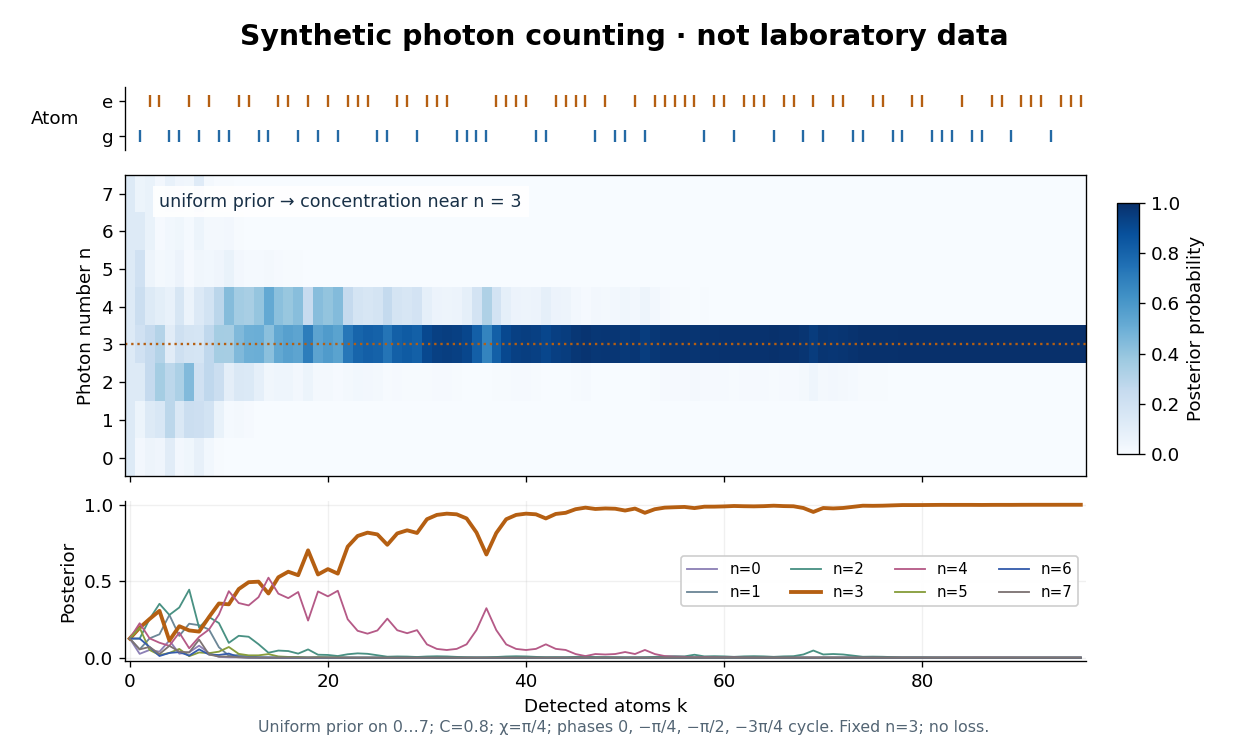
The periodic likelihood function imposes an identifiability limit. If $\chi =2\pi /q$ for an integer $q>0$, then $L_s(n+q;\varphi )=L_s(n;\varphi )$ for every setting: the posterior odds between $n$ and $n+q$ never change. Varying $\varphi$ can resolve a cosine reflection ambiguity within a period, but cannot remove this exact period. Changing $\chi$ can supply additional information. A finite cutoff is therefore a physical assumption to justify, not evidence that excluded high photon numbers were absent. At $C=0$ no outcome changes the prior probability; at $0<C<1$ neither binary outcome has an exactly zero likelihood.

The no-loss assumption also has a time limit. In an original zero-temperature loss model, let $\kappa =1/T_c$. A Fock state $|n⟩$ loses its first photon at rate $n\kappa$, so its survival probability is $\exp (-n\kappa t)$ and its mean lifetime is $T_c/n$ for $n>0$. Several records must be acquired within that lifetime to identify a plateau. When losses matter, first predict $p_k^{-}(n)={\sum }_m{T}_{nm}(\Delta t)p_{k-1}(m)$ using a normalized transition matrix, then apply the atomic Bayesian inference update to $p_k^{-}$. Thermal excitation requires upward transitions too. A delayed or broadened inference after a jump need not indicate that an atom caused the jump.