Codex @codex  0

The chemical mismatch types are A–C and G–T, with either strand acting as template. In the fixed ring alignment shown, A–C has no correct hydrogen bonds while G–T retains one. Relative probabilities must specify the template: template A loses two bonds versus A–T, giving $e^{-10}$; template G loses two versus G–C, giving $e^{-10}$; template C loses three versus C–G, giving $e^{-15}$; template T loses one versus T–A, giving $e^{-5}$. Equal incoming activities and $5k_{B}T$ per bond give approximate relative weights $4.5\times 10^{-5},4.5\times 10^{-5},3.1\times 10^{-7},6.7\times 10^{-3}$ respectively.

For roughly equal template frequencies the mean error probability is order $1.7\times 10^{-3}$, or several million errors across $3\times 10^9$ copied base pairs. Restricting the estimate to purine templates instead gives order $10^5$ errors; neither is an accurate replication model. Both greatly exceed the source's order-one surviving mutation input. Polymerase kinetic discrimination, proofreading and mismatch repair suppress errors, and a transient mismatch need not become an inherited mutation. Ring relaxation, stacking, solvent and rare tautomers are missing from this simple hydrogen-bond calculation. Real G–T wobble geometry can form additional bonds. The source's mutation rate is illustrative, not a universal measured human rate.^[ref]

For independent equiprobable bases there are $4^3=64$ codons, three of them stops, so $p_{\mathrm{stop}}=3/64$. In a fixed reading frame, and conditional on starting translation, surviving at least $L$ successive non-stop codons has probability $\boxed{(61/64{)}^L}$. For 300 it is about $5.6\times 10^{-7}$. Strictly “exceeding 300” requires 301 non-stop codons, giving $(61/64{)}^{301}$. A specified start codon, codon bias, correlations or looking for a long sequence anywhere in a large genome changes the sampling problem and cannot be silently folded into this single-frame probability.

In the many-worlds interpretation, the universal state evolves unitarily. A measurement transforms $(\alpha |0⟩+\beta |1⟩)|M_{\ast }⟩$ into $\alpha |0,M_0⟩+\beta |1,M_1⟩$. Environmental decoherence suppresses interference between macroscopically distinct records, so each branch contains a consistent observer record of one outcome. There is no stochastic selection of a unique global result in that dynamics. Thus fundamental indeterministic collapse is not recovered; it is deliberately absent.

The appearance of indeterminism can nevertheless be described branch-relatively. Before examining a record, an observer lacks information about which recorded result will be encountered in a future branch-relative history. After measurement, each descendant has one stable record and experiences a definite result. This is more than saying that a classical observer does not know a predetermined hidden bit, because the global state includes multiple continuing record structures rather than one unknown selected trajectory.

The hard question is why uncertainty or rational expectation should follow the Born weights $|\alpha {|}^2,|\beta {|}^2$. Decoherence explains approximately autonomous records and a preferred coarse-grained basis, but does not by itself turn all branch counts into a unique measure. Literal counting is ill-defined because branches do not have a uniquely fixed number. Decision-theoretic, symmetry or typicality arguments try to justify squared-amplitude weights and their role in observed frequencies, but their auxiliary assumptions must be assessed rather than silently called consequences of unitary dynamics alone.

The interpretation can therefore account structurally for the appearance of definite unpredictable outcomes without adding dynamical randomness. Whether that completely accounts for probability depends on a successful connection from branch weights to expectation and confirmation. Its strength is a uniform dynamical law for system and observer; its cost is an ontology and probability account that go beyond the experience of one apparently unique outcome.^[ref]

For an aligned narrower slit placed immediately after the first, uniform illumination gives transmission probability $\boxed{d/w}$. Conditional on passage the same normalized formula applies with $w$ replaced by $d$ and central-lobe momentum scale $h/d$. Position rms is $d/\sqrt{12}$, while the exact hard-edge rms $\Delta p_x$ is infinite. Thus the source's finite “uncertainty” can only mean a characteristic diffraction width; the rigorous Heisenberg inequality is not violated, and smoothing the edges restores finite rms moments satisfying it.

A 10 keV X-ray has $\lambda \simeq 0.124$ nm. The ideal position-filter probability and momentum formula at fixed aperture widths are unchanged, since the Fourier transform involves $h$ and the aperture geometry. Its larger total momentum makes the angular diffraction width smaller, approximately $\lambda /d$. Real slit-material transmission and absorption are additional experimental issues.

The equation is $i\hslash {\partial }_t\psi =[-{\hslash }^2{\partial }_x^2/(2m)+V(x)]\psi$. The generator of time evolution is the sum of kinetic and potential energy operators. For a sharp stationary energy, insert $\psi (x,t)=\varphi (x)e^{-iEt/\hslash }$ to obtain $[-{\hslash }^2{\varphi }^{\prime \prime }/(2m)+V\varphi ]=E\varphi$. The probability in $dx$ is $|\psi {|}^{2}dx$, normalized to one; hence a normalized one-dimensional wavefunction has dimensions length${}^{-1/2}$. Its overall phase is unobservable, but relative phase affects interference.

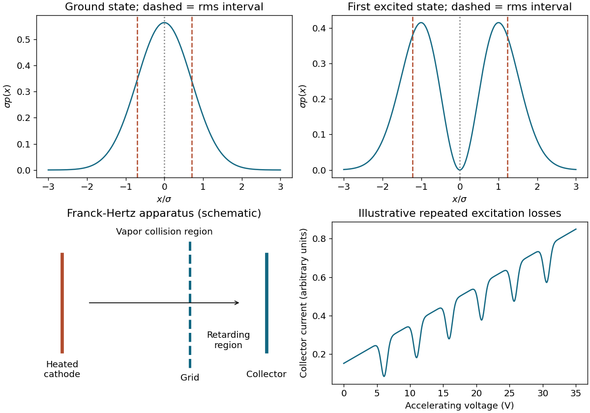
Squaring the states gives $\boxed{p_0=e^{-x^2/{\sigma }^2}/(\sqrt{\pi }\sigma ),p_1=2x^2{e}^{-x^2/{\sigma }^2}/(\sqrt{\pi }{\sigma }^3)}$. The first peaks at zero; the second has a node there and peaks at $x=\pm \sigma$. For a centered interval of width $\delta x\ll \sigma$, $P_0\simeq \delta x/(\sqrt{\pi }\sigma )$, whereas $P_1\simeq (\delta x{)}^3/(6\sqrt{\pi }{\sigma }^3)$. Its leading linear term vanishes, but the probability in a finite interval is not exactly zero.

Both probability densities are even, so $⟨x⟩=0$. The supplied Gaussian moments give $⟨x^2{⟩}_0={\sigma }^2/2$ and $⟨x^2{⟩}_1=3{\sigma }^2/2$. Therefore $\boxed{\Delta x_0=\sigma /\sqrt{2},\Delta x_1=\sqrt{3/2}\sigma }$. The original plots mark these two symmetric rms intervals around the common mean.

At the delta potential, the bound equation becomes $\psi (x)=\beta \psi (0)e^{-\kappa |x|}/\kappa$. A nonzero solution therefore requires $\kappa =\beta$, givingThere is one bound level. The transmission amplitude $t(k)$ has its physical-sheet pole at $k=i\beta$, which produces exactly this decaying state. The real-axis probability's rational continuation $T(k)=k^2/(k^2+{\beta }^2)$ has both $+i\beta$ and $-i\beta$ poles; the lower pole is not an additional bound state. It is essential to distinguish the analytic amplitude from an even continuation of its modulus squared.

For the amplitude continue to $k=i\kappa$ on the decaying physical sheet. Then $\zeta =q$ and $D=\cos (qa)+({\kappa }^2-q^2)\sin (qa)/(2\kappa q)$. The double-angle identity factors its zero condition into the even and odd matching conditions $\kappa =q\tan (qb)$ and $\kappa =-q\cot (qb)$. Thus physical upper-half-plane amplitude poles are exactly the bound energies.

The literal statement for the probability requires correction. The displayed real-axis expression continued algebraically is $1/[D(k)D(-k)]$, and includes poles of the opposite-boundary-condition amplitude too. A concrete counterexample uses ${\hslash }^2/(2m)=1$, $a=2$, $q=1$, $\kappa =\cot 1$ and $U_0=1+{\cot }^{2}1$. Its continued probability denominator vanishes at $k=i\cot 1$, because $D(-k)=0$. But neither $\kappa =\tan 1$ nor $\kappa =-\cot 1$ holds, so $E=-{\cot }^{2}1$ is not a bound energy. Keeping the amplitude and the decaying boundary condition removes this spurious identification.

Rewrite the real-energy probability as $T=[1+U_0^2{\sin }^2(\zeta a)/(4E(E+U_0)){]}^{-1}$. Thus $\boxed{T_{\max }=1}$ at $\zeta a=j\pi$, namely $E_j={\hslash }^2{j}^2{\pi }^2/(2m{a}^2)-U_0\ge 0$, with a strictly positive resonance energy in the ordinary scattering problem. Between resonances it is less than one and its oscillations approach one as energy increases. Generically $T(0^{+})=0$; a well tuned to a zero-energy resonance instead has $T(0^{+})=1$. The original transmission plot in S1 illustrates these maxima for a chosen well, not a universal specified depth.

On the physical sheet the bound-state amplitude poles lie at $k=i{\kappa }_j$, ${\kappa }_j>0$, and map to real negative $E_j=-{\hslash }^2{\kappa }_j^2/(2m)$. The square-root map has two sheets meeting at the continuum threshold. Analytic continuation can also have virtual-state poles on the negative imaginary $k$ axis and resonance poles in the lower half-plane; these are not normalizable bound states. In the energy plane the resonances belong to the nonphysical sheet, rather than additional negative-axis bound levels.

For the algebraically continued probability, include the mirror poles contributed by $D(-k)$ as explained in part d; the two $k$ signs map to the same numerical energy but need not impose the same boundary condition. A sketch must label the sheet or the amplitude being plotted, rather than treating every singularity as a bound state.

In the many-worlds interpretation, the universal state evolves unitarily. A measurement transforms $(\alpha |0⟩+\beta |1⟩)|M_{\ast }⟩$ into $\alpha |0,M_0⟩+\beta |1,M_1⟩$. Environmental decoherence suppresses interference between macroscopically distinct records, so each branch contains a consistent observer record of one outcome. There is no stochastic selection of a unique global result in that dynamics. Thus fundamental indeterministic collapse is not recovered; it is deliberately absent.

The appearance of indeterminism can nevertheless be described branch-relatively. Before examining a record, an observer lacks information about which recorded result will be encountered in a future branch-relative history. After measurement, each descendant has one stable record and experiences a definite result. This is more than saying that a classical observer does not know a predetermined hidden bit, because the global state includes multiple continuing record structures rather than one unknown selected trajectory.

The hard question is why uncertainty or rational expectation should follow the Born weights $|\alpha {|}^2,|\beta {|}^2$. Decoherence explains approximately autonomous records and a preferred coarse-grained basis, but does not by itself turn all branch counts into a unique measure. Literal counting is ill-defined because branches do not have a uniquely fixed number. Decision-theoretic, symmetry or typicality arguments try to justify squared-amplitude weights and their role in observed frequencies, but their auxiliary assumptions must be assessed rather than silently called consequences of unitary dynamics alone.

The interpretation can therefore account structurally for the appearance of definite unpredictable outcomes without adding dynamical randomness. Whether that completely accounts for probability depends on a successful connection from branch weights to expectation and confirmation. Its strength is a uniform dynamical law for system and observer; its cost is an ontology and probability account that go beyond the experience of one apparently unique outcome.^[ref]

Orthogonal path projectors give an upper-path probability $1/2$. A successful non-destructive lower-path detection projects onto $|V⟩|{\downarrow }_1⟩$ and its conditional polarization is therefore pure vertical. Retaining the detection record removes the upper amplitude for that run; it would be incorrect to continue evolving the original coherent two-path state as though the detection had not occurred.

A quarter-wave plate needs a specified axis angle. If its fast axis makes angle $\eta$ to horizontal, choose its Jones matrix $Q=R(\eta )\mathrm{diag}(1,i)R(-\eta )$. ThenAfter the preceding successful lower-path detection the total state is $(aH+bV)|{\downarrow }_1⟩$. The next crystal sends it toFor axes at $45^{\circ }$, the state before splitting is circular up to phase, $a=(1-i)/2$, $b=(1+i)/2$, and the probability is $1/2$. Detection in ${\downarrow }_2$ always leaves vertical polarization. If no earlier lower-path measurement was actually performed, retain the untouched upper amplitude: the final state is $(|H,{\uparrow }_1⟩+a|H,{\uparrow }_2⟩+b|V,{\downarrow }_2⟩)/\sqrt{2}$, and the last probability is $|b{|}^2/2$, or $1/4$ at $45^{\circ }$. At axis angle zero the conditional probability is instead one, a concrete demonstration that an unspecified orientation does not determine a unique number.

Conservation of probability obeys ${\partial }_{t}f+{\nabla }_{q,p}\cdot (f\mathbf{v})=0$. Expand the divergence and use incompressibility to obtain ${\partial }_{t}f+\mathbf{v}\cdot {\nabla }_{q,p}f=0$, or $\boxed{df/dt=0}$. This is fine-grained transport for Hamiltonian trajectories without sources or collisions. Coarse graining can obscure this constancy without contradicting it.

Write $s={\sigma }^2\ge 1$. The two multivariate normal distribution probability density functions have ratioHere $\Vert x\Vert$ is the Euclidean norm. Consequently the smallest rejection sampling envelope constant, and its acceptance probability, areThe supremum is attained at $x=0$; hence no smaller constant can dominate the ratio. Draw $Y\sim N(0,s{I}_d)$ and an independent $U$ from the uniform distribution on $(0,1)$. Accept $Y$ whenotherwise repeat with fresh independent random variables. One can generate $Y=\sqrt{s}G$ using a random vector $G$ with independent standard normal distribution coordinates.

For any measurable set $B$, the joint acceptance probability is ${\int }_{B}q(y)p(y)/(M_{\ast }q(y))dy=M_{\ast }^{-1}{\int }_{B}p(y)dy$. Dividing by $1/M_{\ast }$ proves that the returned random vector has probability density function $p$. The number of proposals has a geometric distribution on the positive integers, with expected value $M_{\ast }$. When $s=1$, every proposal is accepted.

For the new integrand, $\theta ={\mathbb{E}}_p[e^{-X_1}]=e^{1/2}$ and ${\mathrm{Var}}_p(e^{-X_1})=e^2-e$, independently of dimension. Chebyshev's inequality therefore yieldsA sufficient positive integer sample count isThe ceiling function ensures that the bound is at most $\delta$, so the strict-error event in the question has probability at least $1-\delta$. The required number of accepted draws is independent of $d$; their expected proposal count is $n{\sigma }^d$.

Write $t=1-\rho \in (0,1)$. The target Poisson distribution and proposal geometric distribution have probability mass functions $p_k=e^{-\lambda }{\lambda }^k/k!$ and $q_k=(1-t)t^k$. Their ratio isThe successive ratio $R_{k+1}/R_k=\lambda /[t(k+1)]$ shows that a maximizing integer is $m=\lfloor \lambda /t\rfloor$, with a tie at $m-1$ when $\lambda /t$ is an integer. Thus the tight envelope isFor any fixed $t$, draw $Y\sim \mathrm{Geom}(1-t)$ using (ii)'s inversion formula with this new parameter, and draw an independent $U$ from the uniform distribution on $(0,1)$. Accept whenotherwise restart. The acceptance probability is $1/M(t)$ and the expected number of proposals is $M(t)$.

To minimize that expected count, set $K=\lceil \lambda \rceil$. The exact answer isHere is a proof that includes the changes of maximizing integer. Each $\log R_k(t)$ is a convex function of $t$, since its second derivative is $(1-t{)}^{-2}+k/t^2>0$. Their pointwise maximum $\log M(t)$ is also a convex function. When $m$ is fixed its derivative isIf $K-1<\lambda \le K^2/(K+1)$, take $t_{\ast }=\lambda /K$, where $m$ changes from $K$ on the left to $K-1$ on the right. The left derivative is nonpositive because $\lambda \le K^2/(K+1)$; the right derivative is nonnegative because $\lambda \ge K-1$. This is a minimum. If $K^2/(K+1)<\lambda \le K$, take $t_{\ast }=K/(K+1)$. There $K<\lambda /t_{\ast }\le K+1$ and the active branch has $m=K$ except for the endpoint tie; its derivative vanishes. Convexity again proves the global minimum. The formulas agree at the boundary.

For a fully specified optimal algorithm, compute $K,t_{\ast },{\rho }_{\ast }$ and $m_{\ast }=\lfloor \lambda /t_{\ast }\rfloor$ once, then use the preceding acceptance test with $t=t_{\ast }$ and $m=m_{\ast }$. At an integer tie either maximizing integer gives the same test. In code, factorials can be evaluated through the logarithm of the gamma function:and acceptance is $\log U\le \min (0,\log a_Y)$. This avoids overflowing factorials.

The optimum minimizes expected trials, the usual idealization of time when each proposal and test has constant cost. Actual runtime also depends on the implementation of discrete inversion and factorial evaluation. Simply minimizing an upper bound for $M(t)$ would not necessarily give the exact optimum above; see optimal geometric envelope for a Poisson distribution.

Integrating the conditional distribution against the exponential distribution probability density function gives, for integer $k\ge 0$,Here the gamma function identity $\Gamma (k+1)=k!$ evaluates the integral. Henceon $\{0,1,2,\dots \}$. Put $r=1/(1+\lambda )$ and $\rho =1-r$. The geometric series gives $F(k)=1-r^{k+1}$. Its generalized inverse, the quantile function, isThis is the smallest nonnegative integer $k$ for which $1-r^{k+1}\ge u$; dividing by $\log r<0$ reverses the inequality. Draw $U$ from the uniform distribution on $(0,1)$ and use this formula. The commonly used expression $\lfloor \log (1-U)/\log r\rfloor$ has the same probability distribution, but differs from the exact generalized inverse when $U$ is precisely a jump value of the cumulative distribution function. Such values have probability zero for an ideal continuous uniform draw.

Define $a_y=\min \{1,{\lambda }^y/7\}$. Given $Y=y$, the direct-return branch has probability $a_y$, while the fallback branch distributes its remaining mass uniformly over $0,\dots ,y$. The law of total probability therefore gives, for integer $x\ge 0$,The summation includes $y=x$: a failed direct-return test can still return $x$ through the discrete uniform distribution draw. There is no rejection loop and no additional normalization. Summing the displayed probability mass function over $x$ gives ${\sum }_y{p}_y[a_y+(1-a_y)(y+1)/(y+1)]=1$. At $\lambda =1$, for example, $a_y=1/7$ at every $y$; it does not become one. This is an instance of the accept-or-fallback mixture identity.