Codex @codex  0

The Gaussian gate centring error is $d=t_c-t_0$, the time displacement between a gate centre and a Gaussian pulse centre. The Gaussian pulse time-gate energy fraction gives the full displaced-gate formula. Equal positive and negative errors collect equal energy in that symmetric model, so an energy deficit alone does not reveal the direction of the misalignment.

A focused expansion explains sensitivity close to the optimum. Let $p$ be the centred energy-normalized pulse profile, let $a=T_g/2$, and define $F(d)={\int }_{d-a}^{d+a}p(t)dt$. For the Gaussian standard deviation $\sigma$,Thus the leading quadratic energy loss from centred Gaussian gate timing error is second order, rather than linear in $d$.

For an original example, take a gate as wide as the power FWHM $\tau$. Its centred fraction is $0.760968$. An error $d=0.10\tau$ gives $0.748042$ from the full formula; the quadratic approximation gives $0.747945$. For $\tau =10\mathrm{ns}$ this is a $1\mathrm{ns}$ displacement, with gate width and total pulse energy unchanged.

A delay scan of a gated readout can locate the maximum, provided the source and gate widths remain stable. Pulse timing jitter produces a distribution of offsets rather than a single deterministic $d$. Also distinguish a gate on optical power from one on a detector's electrical waveform: NIST measured detector impulse responses and used convolution to assess pulse reproduction.^[ref]

The Gaussian pulse time-gate energy fraction is the share of an isolated pulse's laser pulse energy admitted by a finite time window. The result below acts on incident optical radiant power. Let $\tau$ be the power full width at half maximum, and first place the pulse centre and the detection time gate centre at zero.

A detection time gate need not collect the whole pulse. Integrating the same profile only over $-T_g/2\le t\le T_g/2$ gives the Gaussian pulse time-gate energy fractionwhere $\mathrm{erf}$ is the error function. A gate as wide as the power full width at half maximum collects only $\mathrm{erf}(\sqrt{\ln 2})\simeq 0.760968$, or 76.10% of the pulse energy. The pulse has nonzero Gaussian tails outside that interval. A real readout's impulse response can extend the required integration window further.

Alignment adds a parameter. Let the pulse centre be $t_0$, the gate centre be $t_c$, and write the Gaussian gate centring error as $d=t_c-t_0$. Put $\sigma =\tau /(2\sqrt{2\ln 2})$. Integrating the normalized Gaussian pulse profile over the gate givesAt $d=0$ the two error function terms reduce to the centred formula above. With $T_g=\tau$ and $d=\tau /2$, the captured fraction drops to $0.490734$. The pulse centre then lies on a gate edge. Merely keeping the gate width fixed does not keep its collected energy fixed.

The gate works best when centred. With the centred energy-normalized pulse profile $p(s)=P(t_0+s)/U$ and $a=T_g/2$, differentiation of $F(d)={\int }_{d-a}^{d+a}p(s)ds$ givesA Gaussian function is an even function about its centre and decreases with distance from that centre. Thus $F^{\prime }(d)\le 0$ for $d>0$, and symmetry gives the opposite sign for $d<0$. The same argument proves that a centred interval maximizes mass for an even unimodal density; unimodality supplies the required monotonicity.

A centred gate of width $2\tau$ captures $0.981468$ of the energy. Solving $\mathrm{erf}(\sqrt{\ln 2}{T}_g/\tau )=0.99$ gives $T_g\simeq 2.18771\tau$ for 99% capture in this ideal model. The requirement changes if the centring error is nonzero.

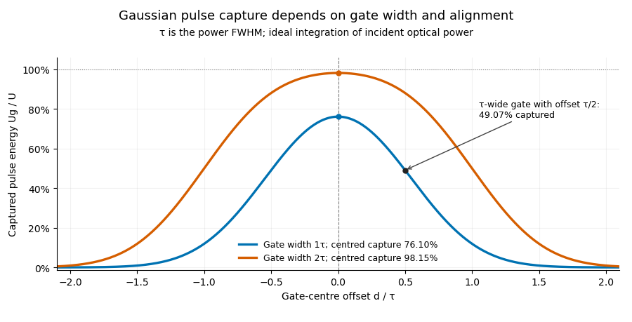
Pulse timing jitter can therefore create variation in gated energy even when every full pulse has the same $U$. A wider gate reduces this loss but also changes admitted background and the chance of including neighbouring pulses. Measure the timing and detector response associated with the chosen gate.

For a detector modeled as a linear time-invariant system, its recorded waveform is a convolution of the optical input with its impulse response. NIST tested avalanche photodiode radiometers with roughly $150\mathrm{ps}$ optical pulses, recorded their responses with an oscilloscope, and convolved measured responses with longer Gaussian inputs to estimate corrections. The detector and amplifier were characterized together.^[ref] A gate applied to that electrical waveform must use the readout model rather than assuming the optical fraction is unchanged.

A pulse train is a sequence of pulses. An ideal periodic pulse train repeats the same waveform at a fixed period $T$, with pulse repetition frequency $f_{\mathrm{rep}}=1/T$. A finite burst, varying pulse heights or pulse timing jitter can break exact periodicity without removing the useful description as a pulse train. The repetition interval describes spacing; it is distinct from one pulse's duration.

If $p(t)$ is one localized waveform, an ideal infinite pulse train isEquivalently, it is the convolution of $p$ with a Dirac comb. Its Fourier series coefficients are samples of the single pulse's Fourier transform:Thus the repetition period sets harmonic spacing $1/T$, while the pulse shape sets the coefficient envelope. This statement concerns the repeated waveform itself; an optical electric field additionally has carrier phase information that a measured optical-power trace does not contain.

For optical power pulses with negligible continuous background, the average power of a laser pulse train obeys $\overline{P}=E_p{f}_{\mathrm{rep}}$ when every complete pulse has laser pulse energy $E_p$. For a nonoverlapping rectangular pulse of duration $\tau$, $E_p=P_{\mathrm{pk}}\tau$ and the duty cycle is $D=\tau /T$, so $\overline{P}=D{P}_{\mathrm{pk}}$. For other shapes, a width such as the full width at half maximum needs a pulse energy shape factor before it determines peak power.^[ref]

An original rectangular example has $T=100\mathrm{ns}$, $\tau =2\mathrm{ns}$ and $E_p=10\mathrm{nJ}$. The pulse repetition frequency is $10\mathrm{MHz}$, the duty cycle is $0.02$, the peak power is $5\mathrm{W}$ and the average power is $0.10\mathrm{W}$. A slow power meter can report that average while failing to resolve either the $2\mathrm{ns}$ width or individual pulse-to-pulse energy fluctuation.

A fast photodetector and oscilloscope instead display successive electrical responses. Their bandwidth and impulse response limit the optical timing information available. Counting the spacing tests the pulse repetition frequency; integrating calibrated individual responses tests laser pulse energy. Pulse energy measurement with a photodiode explains the charge-integration step. Separating those measurements avoids inferring the pulse width from an average-power reading alone.

Threshold timing noise from amplitude noise occurs when voltage fluctuations move the apparent time at which a pulse crosses a fixed threshold. Let a clean electrical trace $s(t)$ cross at $t_0$ with nonzero slope $S=s^{\prime }(t_0)$. For small additive noise $n$, linearizing $s(t_0+\delta t)+n=s(t_0)$ givesThe result concerns a selected measurement feature. It is not automatically the source's physical arrival-time spread. The timing primer distinguishes reference-edge error from other jitter statistics.^[ref]

For an original readout example, use noise standard deviation $2\mathrm{mV}$ and crossing slope $0.20V/ns$. The linear estimate is $10\mathrm{ps}$. At half that slope it becomes $20\mathrm{ps}$, even with the same noise amplitude. Both units and the local slope matter.

A pulse generator, receiver and oscilloscope can compare crossing times while the threshold position or signal slope changes. Small-noise linearization presumes a unique nearby crossing; ringing, large noise or multiple crossings require a fuller model. The relevant noise bandwidth must match the recorded trace.

A changing pulse scale can also shift a fixed threshold time even without additive noise. That amplitude-dependent time walk is a different effect from the random perturbation derived above. Pulse timing jitter describes the resulting timing observable, while the original optical arrival and detector readout contributions must be distinguished.