A pulse is a localized disturbance that passes a fixed location during a bounded or effectively bounded time interval. A travelling wave pulse may be written with localized . Its width and peak amplitude describe its extent and size; a wave packet additionally emphasizes a carrier and an envelope.
A pulse train is a sequence of pulses. An ideal periodic pulse train repeats the same waveform at a fixed period , with pulse repetition frequency . A finite burst, varying pulse heights or pulse timing jitter can break exact periodicity without removing the useful description as a pulse train. The repetition interval describes spacing; it is distinct from one pulse's duration.
If is one localized waveform, an ideal infinite pulse train isEquivalently, it is the convolution of with a Dirac comb. Its Fourier series coefficients are samples of the single pulse's Fourier transform:Thus the repetition period sets harmonic spacing , while the pulse shape sets the coefficient envelope. This statement concerns the repeated waveform itself; an optical electric field additionally has carrier phase information that a measured optical-power trace does not contain.
For optical power pulses with negligible continuous background, the average power of a laser pulse train obeys when every complete pulse has laser pulse energy . For a nonoverlapping rectangular pulse of duration , and the duty cycle is , so . For other shapes, a width such as the full width at half maximum needs a pulse energy shape factor before it determines peak power.[ref]
Average and Peak Power - A Tutorial by Newport. Photonics Technical Note1, one-page rectangular-pulse diagram and average-power/duty-cycle equations
An original rectangular example has , and . The pulse repetition frequency is , the duty cycle is , the peak power is and the average power is . A slow power meter can report that average while failing to resolve either the width or individual pulse-to-pulse energy fluctuation.
A fast photodetector and oscilloscope instead display successive electrical responses. Their bandwidth and impulse response limit the optical timing information available. Counting the spacing tests the pulse repetition frequency; integrating calibrated individual responses tests laser pulse energy. Pulse energy measurement with a photodiode explains the charge-integration step. Separating those measurements avoids inferring the pulse width from an average-power reading alone.
Pulse timing jitter describes variation of pulse arrival times relative to a stated timing reference. Choose a reproducible pulse feature and reference instants ; define errors . One measure is their standard deviation . Edge-time error relative to an ideal reference differs from variation of successive periods or cycle-to-cycle differences; the primary timing guide distinguishes these measurements.[ref]
Digital Design Debugging Guide by Tektronix. Picking out Jitter, Diagram5 and statistical discussion, printedpp.12–14
For an original distribution, let each error equal , where is equally likely to be or . The mean delay is and . The root mean square error about zero is instead . A fixed delay changes the mean without increasing the spread. None of these numbers is the individual pulse's duration.
A fast photodetector, reference timing signal and oscilloscope can measure a selected arrival feature. A fixed electrical threshold can also turn amplitude/readout noise into an apparent time change, producing threshold timing noise from amplitude noise. Specify the reference, feature, observation duration and measurement response. A fitted or recovered reference can absorb some timing variation, changing the reported residual.
Timing variation can become gated-energy variation even at constant full pulse energy. The Gaussian gate centring error provides one quantitative model, distinct from pulse-to-pulse energy fluctuation of complete pulses.
Threshold timing noise from amplitude noise occurs when voltage fluctuations move the apparent time at which a pulse crosses a fixed threshold. Let a clean electrical trace cross at with nonzero slope . For small additive noise , linearizing givesThe result concerns a selected measurement feature. It is not automatically the source's physical arrival-time spread. The timing primer distinguishes reference-edge error from other jitter statistics.[ref]
Digital Design Debugging Guide by Tektronix. Picking out Jitter, Diagrams5–6
For an original readout example, use noise standard deviation and crossing slope . The linear estimate is . At half that slope it becomes , even with the same noise amplitude. Both units and the local slope matter.
A pulse generator, receiver and oscilloscope can compare crossing times while the threshold position or signal slope changes. Small-noise linearization presumes a unique nearby crossing; ringing, large noise or multiple crossings require a fuller model. The relevant noise bandwidth must match the recorded trace.
A changing pulse scale can also shift a fixed threshold time even without additive noise. That amplitude-dependent time walk is a different effect from the random perturbation derived above. Pulse timing jitter describes the resulting timing observable, while the original optical arrival and detector readout contributions must be distinguished.
Pulse duration quantifies a pulse's temporal extent using a stated observable and width convention. A common optical convention is the full width at half maximum of the background-subtracted radiant power profile. The Ansys source documentation explicitly defines its PULSELENGTH parameter as the power-profile FWHM, rather than the width of the electric-field amplitude.[ref]
Plane wave and beam source - Simulation object in Ansys Optics documentation. Frequency/Wavelength tab, Standard source PULSELENGTH definition
For an original example, choose a triangular power pulseIts nonzero support extends from to , giving total support width . Its half-maximum crossings occur at , giving a power FWHM of only . Neither number is wrong when its convention is specified. The pulse energy shape factor additionally relates a chosen width to integrated energy and peak power.
A fast photodetector and oscilloscope record an electrical response to an optical pulse. For a linear response model, the recorded trace is a convolution with the instrument's impulse response; a slow response can broaden the measured feature. The readout width need not equal the optical width. State the observable, background treatment and instrument response when reporting a duration. Pulse energy baseline correction affects where the half-maximum threshold lies, while Gaussian pulse energy and peak power treats the conversion for a specific power-profile family.
Laser pulse energy is the radiant energy carried by one specified laser pulse across a measurement plane. For an isolated pulse whose total radiant power is and whose background is zero,Here is already integrated over the transverse beam area; it is not local irradiance. The unit of is the joule. Radiant exposure instead divides received energy by a receiving area, so a beam's alone does not specify the exposure at its centre. The radiant exposure of a Gaussian beam makes that spatial distinction quantitative.
The Gaussian pulse energy and peak power relation gives when is the power full width at half maximum. The pulse energy shape factor records pulse-shape dependence, while the Gaussian pulse field-envelope width is times the power width.
For an original example, stipulate and a Gaussian pulse power full width at half maximum . Then . Stretching the same model pulse to while keeping unchanged reduces its peak power to . Both curves below integrate to the same energy; their peak heights and widths differ.
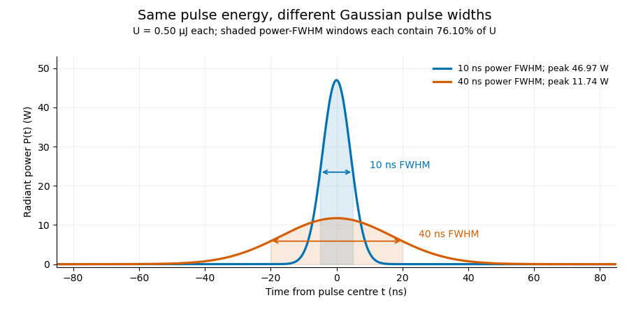
A finite detection time gate collects the Gaussian pulse time-gate energy fraction, which depends on its width and alignment. A centred gate as wide as the power full width at half maximum receives only of , because Gaussian tails extend beyond it. For a -wide gate, a Gaussian gate centring error of reduces capture to .
The average power of a laser pulse train follows by counting complete pulses. If a long observation of duration contains pulses of energies , with negligible edge contributions and no continuous background,Here is the pulse repetition frequency, not the inverse pulse width. An average power readout constrains when is known; it does not resolve pulse-to-pulse energy fluctuation. Identical, well-separated pulses at give average power, even though the stipulated pulses peak near .
If a steady optical background is present, state whether the reported energy includes it. For pulse energy above a measured background , the pulse energy baseline correction uses . Failing to subtract a constant background adds to the inferred energy. This optical-background model is distinct from an offset introduced later by detector electronics.
Historical NIST equipment illustrates what the readouts measure. Its TC-24 reference absorbed the beam in a glass plate, sensed a plate temperature difference with thermocouples, and integrated the thermopile's electric potential difference during beam injection. Before/after readings enabled background subtraction and compensated thermal drift. Counting pulses converted total injected energy to mean pulse energy. The semiconductor pulse photodetector used an integrating amplifier; calibration related the peak output electric potential difference to pulse energy. That electrical peak did not by itself establish optical peak power.[ref]
Calibration Service for Low-level Pulsed-Laser Radiometers at 1.06 µm: Pulse Energy and Peak Power by Rodney W. Leonhardt. §3.5, printed p. 8; §4, printed pp. 9–10: thermal reference, baselines, pulse counting and integrated readout
Pulse energy measurement with a photodiode connects this kind of measurement to collected electric charge; validating the detector response under the actual pulse conditions remains part of that interpretation.Pulse-to-pulse energy fluctuation is variation in the laser pulse energy of successive emitted pulses. For a stationary population with finite variance, its standard deviation is . A finite record supplies an estimate, whose convention should be stated rather than being confused with the uncertainty of the record's mean.
For an original four-pulse record, take measured energies . Their mean is . The sample standard deviation isIts coefficient of variation is 11.55 percent. The root-mean-square deviation of this particular list, using divisor four rather than three, is instead or 10 percent. The definition matters when comparing reported stability figures. The familiar estimate of uncertainty in a mean additionally assumes independent, identically distributed observations; an ordered record alone does not establish that assumption.
A historical NIST stability assessment compared an internal excimer-laser pulse monitor with a pyroelectric laser-energy meter. Its calorimeter integrated a pulse train, so averaging and individual-pulse variation entered different parts of the analysis.[ref]
Calibration Service for Laser Power and Energy at 248 nm by Rodney W. Leonhardt. §6.2, Laser stability, printedp.23
Observed variability also includes readout noise. Separating detector noise from pulse-energy variance requires an appropriate measurement model and independent information about that noise. Detector saturation, drift and correlated pulse errors are not removed merely by collecting a longer record. An average power of a laser pulse train measurement by itself does not resolve this sequence.
Separating detector noise from pulse-energy variance estimates source variability using a model of the readout's own fluctuations. In energy-calibrated units, write . The exact identity isOnly when the covariance vanishes can a separately estimated noise variance be subtracted directly. Covariance terms are part of measurement-model uncertainty propagation, rather than an optional correction.[ref]
For an original independent-noise example, suppose the observed energy standard deviation is and a matched noise-only measurement gives . The inferred source standard deviation is , not . The source contributes of the observed variance in this stipulated model.
A noise-only record should use comparable gain, integration gate and reset conditions. Background subtraction removes an estimated mean, not the random variance remaining around it. Amplifier clipping, unmatched integrator reset or signal-dependent detector noise can invalidate an additive independent-noise model. A negative variance difference is not a physical negative source variance; it can indicate estimation uncertainty or mismatched assumptions.
Splitting pulses between two independently characterized readouts can provide a two-channel covariance estimate of pulse-energy variance under additional noise assumptions. Shared electronics noise and common drift must still be assessed; independence cannot be established just by using two detectors.
A two-channel covariance estimate of pulse-energy variance uses the component shared by paired readouts to estimate source fluctuations. In a stipulated linear model let and , with calibrated nonzero gains. If both noise terms are uncorrelated with and with each other,This follows by expanding the covariance. Correlation assumptions are essential measurement-model inputs; the uncertainty guide retains covariance terms explicitly.[ref]
For an original example, choose , and measured covariance . The inferred source variance is , giving a standard deviation of . Independent readout-noise variances and would give total variances and while preserving that cross-covariance.
But a shared noise covariance of raises the observed cross-covariance to . Ignoring it would infer a source standard deviation of , about too high.
A split-beam experiment records both channels for the same pulses, checks gains and measures dark or independent-input controls for correlated electronics. NIST's calibrated splitting apparatus supplies an example of the optical geometry, not a claim that it used this covariance estimator.[ref]
Calibration Service for Low-level Pulsed-Laser Radiometers at 1.06 µm: Pulse Energy and Peak Power by Rodney W. Leonhardt. §3.4, calibrated beam splitting
Matching pulse indices, bandwidth and integration windows is part of the proposed model.Pulse energy baseline correction subtracts the estimated non-pulse contribution before integrating a measurement trace. For a trace calibrated in power units over a gate ,The estimate must have the same units as the integrated trace. Optical background and a detector-electronics offset enter at different stages of a physical measurement; a voltage offset cannot be subtracted directly from optical power without a response calibration.
An original drift example takes a gate. Suppose pulse-free observations establish a baseline increasing linearly from to across that gate. Its integrated contribution isIf the measured trace integrates to , the corrected estimate is . Subtracting only the initial would yield , with a positive error. This is a baseline-drift bias in pulse-energy integration in a stipulated linear model.
Historical NIST measurements took baselines before and after each run and averaged them to correct background and thermal drift. The leakage-background configuration was specified separately from a pulse injection.[ref]
Calibration Service for Low-level Pulsed-Laser Radiometers at 1.06 µm: Pulse Energy and Peak Power by Rodney W. Leonhardt. §3.5, printedp.8; §7.2, Type B component4, Leakage Effect
Bracketing observations must genuinely represent the non-pulse signal; they cannot include an unrecognized pulse tail. Subtraction also cannot recover energy excluded by a detection time gate or repair a nonlinear detector. The Gaussian pulse time-gate energy fraction quantifies one profile-specific truncation effect.Baseline-drift bias in pulse-energy integration is the systematic energy error caused by using an inaccurate baseline over the integration gate. Relative to the true signal energy in the same gate,This error is separate from energy excluded by the gate. Historical NIST measurements bracketed each run with baseline observations and subtracted their average to compensate background and thermal drift.[ref]
Calibration Service for Low-level Pulsed-Laser Radiometers at 1.06 µm: Pulse Energy and Peak Power by Rodney W. Leonhardt. §3.5; §7.2, Type B component4, Leakage Effect
An original curvature example shows a limit of endpoint bracketing. On , suppose . Both endpoint baselines equal , so their average and the straight interpolation between them coincide. However, the true integrated baseline is . Subtracting the endpoint level over the whole gate therefore givesFor a gate whose endpoints are above its midpoint baseline, this bias is . A true gated signal energy of would be reported as under these assumptions.
Thus quadratic baseline curvature in gated energy integration survives a correction that is exact for a linear baseline. For fixed curvature, the error grows with the cube of gate duration. Additional pulse-free samples can test the baseline model, but pulse tails in those samples can themselves corrupt the estimate. Pulse energy baseline correction supplies the broader measurement context.
Quadratic baseline curvature in gated energy integration describes a baseline whose second time derivative is nonzero over the measurement gate. Averaging only its two endpoint values is exact for a linear baseline but generally not a quadratic one. The baseline-drift bias in pulse-energy integration article derives the resulting endpoint-subtraction error.
A focused correction follows from Simpson's rule. For a quadratic baseline on ,For an original example, take and baseline readings at the beginning, midpoint and end. The integrated baseline is . Endpoint averaging would instead subtract , biasing the inferred signal by .
This Simpson baseline integration for pulse-energy correction needs a genuine baseline at the midpoint. A sample taken during the pulse contains signal as well as background. A separate matched blank run or independently characterized reference can supply additional information; treating a contaminated pulse sample as baseline does not improve the correction. If the midpoint estimate is biased by , the Simpson integral is biased by .
Historical NIST measurements used before/after baselines and averaged them for background and thermal-drift compensation.[ref]
Calibration Service for Low-level Pulsed-Laser Radiometers at 1.06 µm: Pulse Energy and Peak Power by Rodney W. Leonhardt. §3.5; §7.2, Leakage Effect
The three-point quadratic example is an independent mathematical extension, not a description of that apparatus's processing.Simpson baseline integration for pulse-energy correction subtracts a three-point estimate of integrated background from a measured gate integral. For a baseline on , Simpson's rule givesIt is exact for a quadratic or cubic baseline, provided the three values represent background rather than pulse-contaminated samples. For a four-times differentiable baseline, the remainder is for some .[ref]
3.5 Quadrature, subsection (ii) Simpson’s Rule. equation3.5.6, elementary rule and fourth-derivative remainder
For an original chosen quadratic background, take with beginning, midpoint and end values , and . Its integrated baseline is , whereas endpoint averaging would give . A raw gate integral of therefore gives after the three-point correction. Overestimating only the midpoint by would subtract an extra .
The uncertainty of a three-point baseline integral is separate from its quadrature error. With baseline-sample covariance matrix and , its variance is . Independent samples of common standard uncertainty give ; a perfectly shared additive baseline error of the same uncertainty gives instead. Covariance terms cannot be discarded.[ref]
A matched blank acquisition or independently measured background can supply the midpoint. Historical NIST pulse-energy apparatus used before/after baselines for background and thermal-drift compensation.[ref]
Calibration Service for Low-level Pulsed-Laser Radiometers at 1.06 µm: Pulse Energy and Peak Power by Rodney W. Leonhardt. §3.5, reference-standard processing; §7.2, Leakage Effect
The three-point example is an original extension, not a claim about that instrument's processing. Higher polynomial exactness does not compensate for an incorrectly identified baseline.The uncertainty of a three-point baseline integral depends on both the sample uncertainties and their correlations. With a known fixed gate duration , Simpson baseline integration for pulse-energy correction uses the linear combinationIf is the covariance matrix of the baseline estimates, thenFor fixed weights this variance identity is exact; it does not require Gaussian errors. Its use as a complete measurement uncertainty still requires an adequate baseline model. The general covariance propagation rule retains these cross terms.[ref]
An original equal-precision model assigns each sample standard uncertainty and common pairwise correlation coefficient , with . Substitution givesFor and , independent samples give . At this rises to ; a perfectly common additive error gives . Three readings under one uncertain offset need not behave like independent measurements.
The final corrected pulse integral has another covariance. If is the raw gate integral and , thenThe covariance between a raw pulse integral and its baseline correction matters when both share a readout offset. If that offset is , it contributes to both and and cancels exactly in their difference. Treating these appearances as independent would invent uncertainty.
Use repeated matched blank acquisitions to estimate the relevant covariance structure, keeping the gate and readout sequence comparable. A contaminated midpoint, an inadequate baseline shape or uncertain timing adds effects outside the fixed-weight sample-noise calculation. Numerical quadrature exactness alone does not establish a sound pulse-energy uncertainty budget.
A raw laser pulse energy estimate and its baseline correction can contain the same readout error. Let be the raw gate integral, the estimated integrated background and the corrected result. Linearity of covariance gives the exact identityFor this linear measurement model, the law of propagation of uncertainty is exact whenever the input variances exist. Its general form includes the sensitivity coefficients and covariance terms.[ref]
Guidelines for Evaluating and Expressing the Uncertainty of NIST Measurement Results by Barry N. Taylor and Chris E. Kuyatt. Appendix A, equation A-3
Positive covariance reduces the variance of this difference; it would instead increase the variance of a sum.An original shared-offset model makes the mechanism explicit. For fixed gate duration , writewhere is a common additive power-readout offset with standard uncertainty , while and are independent zero-mean energy errors, independent also of . Then , and shared-offset cancellation in a baseline-corrected pulse integral gives . The shared offset contributes no uncertainty to this difference. It need not be small or separately known.
Choose , , and . The shared energy contribution is in each reading. Thus , and , yielding . Incorrectly discarding the covariance gives .
Cancellation weakens if the offset changes between acquisitions. Replace by two offsets with the same standard uncertainty and correlation coefficient . Under the same independent residual-error assumptions,At , the chosen example gives . A baseline taken far away in time cannot simply be assigned the covariance of an unchanged offset.
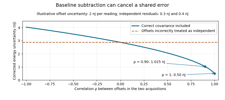
Shared baseline errors cancel according to their correlation
. Original numerical model with a 2 nJ offset uncertainty in each acquisition and independent residual uncertainties of 0.3 nJ and 0.4 nJ. The comparison curve incorrectly treats the shared offsets as independent. Details.A sampled implementation has the same structure. If a vector of readings has covariance matrix , and fixed integration weights give and , thenA constant offset cancels when the weights sum to the same gate duration: . This does not justify using pulse-contaminated readings as background. Matched blank sequences, collected with the actual timing, help characterize the needed noise correlations.
The historical NIST TC-24 apparatus used a thermocouple-based absorbing plate and averaged baseline measurements before and after laser injection to compensate background and thermal drift.[ref]
Calibration Service for Low-level Pulsed-Laser Radiometers at 1.06 µm: Pulse Energy and Peak Power by Rodney W. Leonhardt. §3.5, printed p. 8; §7.2, Leakage Effect
The offset model above is an independent illustration, not a reconstruction of that instrument's uncertainty budget.Moment conditions for baseline-drift cancellation specify which polynomial backgrounds a linear measurement removes. Let readings at known times enter the corrected pulse estimate as , with the integration/calibration units included in . A background contributes nothing wheneverSubstitution gives this result directly. The zeroth condition removes a common offset; the first additionally removes linear drift. These conditions concern the actual weights and times, not only the number of background samples.
An original one-bin signal model measures a pulse at , with uncontaminated reference samples at and . UseThe weights sum to zero and have zero first time moment. Constant and linear backgrounds cancel exactly, but a quadratic background leaves bias . With chosen , and , the bias is . Here the pulse is stipulated to occupy the central bin; the formula is not a universal integral estimator for an arbitrary waveform.
Cancellation has a noise cost of polynomial baseline cancellation. For independent equal-variance reading errors , the chosen estimate has variance , even though its constant and linear bias terms vanish. General correlations use instead.[ref]
NIST's historical pulse-energy apparatus used before/after baselines for background and thermal-drift compensation.[ref]
Calibration Service for Low-level Pulsed-Laser Radiometers at 1.06 µm: Pulse Energy and Peak Power by Rodney W. Leonhardt. §3.5, printed p. 8; §7.2, Leakage Effect
The polynomial test above is an original general analysis. Pulse contamination in a reference, uncertain timing or drift outside the assumed polynomial family can leave a residual even when the nominal algebraic conditions hold.The noise cost of polynomial baseline cancellation is the change in random measurement uncertainty when extra background trends are removed. For a linear pulse estimate and reading-error covariance matrix ,The moment conditions for baseline-drift cancellation constrain to reject specified polynomial backgrounds. They do not make the remaining random error vanish.[ref]
For an original comparison, assume a pulse occupies only the central sample and the other samples contain background alone. Three samples at with weights cancel constant and linear backgrounds. Five samples at can instead useThese weights preserve the central signal and have zero moments of orders . For independent reading errors of equal variance , the three-sample variance is , while the five-sample variance isWith and , the standard uncertainties are approximately and . The second design removes quadratic and cubic drift as well, but its larger reference weights increase noise. This compares two specified estimators; it is not a claim that collecting more background data must worsen precision.
NIST's pulse-energy apparatus used before/after baseline measurements for background and thermal-drift correction.[ref]
Calibration Service for Low-level Pulsed-Laser Radiometers at 1.06 µm: Pulse Energy and Peak Power by Rodney W. Leonhardt. §3.5, printed p. 8; §7.2, Leakage Effect
The polynomial comparison above is an original model for choosing such measurements. Choosing minimum-noise weights under baseline moment constraints can exploit additional reference samples and their measured correlations. Pulse leakage into a reference or drift outside the cancelled polynomial family still creates bias.Minimum-noise weights under baseline moment constraints choose a linear pulse estimator with the smallest variance among those that preserve a specified signal and remove specified backgrounds. Write the reading vector as , where is a known signal template, the columns of contain baseline shapes, and the error covariance matrix is positive definite. For , requireColumns in implement the moment conditions for baseline-drift cancellation. The noise cost of polynomial baseline cancellation depends on which feasible weights are chosen.
If the constraint columns are independent, Lagrange multipliers giveFor any feasible perturbation , and , so the variance increases by . This proves the minimum and connects the estimator to generalized least squares. The covariance propagation is the full quadratic form, not a sum that discards correlations.[ref]
For an original one-bin pulse example, use five equally spaced times , a signal present only at the centre, and independent errors of variance . To remove just constant and linear backgrounds, the optimal dimensionless weights are . Their variance is , lower than for the centre and its two nearest references alone. Multiplying the amplitude estimate by a bin duration gives energy variance . Extra uncontaminated references can reduce noise when the cancelled background family stays the same.
The inverse requires genuinely independent constraints. Constraint redundancy in baseline-noise minimization calls for removing redundant columns and checking feasibility; a signal template inside the nuisance span cannot be preserved while that span is rejected. NIST's before/after pulse baselines provide the physical measurement context.[ref]
Calibration Service for Low-level Pulsed-Laser Radiometers at 1.06 µm: Pulse Energy and Peak Power by Rodney W. Leonhardt. §3.5, printed p. 8; §7.2, Leakage Effect
The five-point design is an original idealization and assumes no pulse signal in its reference samples.Constraint redundancy in baseline-noise minimization occurs when some signal-preservation or baseline-rejection conditions are linear combinations of others. In minimum-noise weights under baseline moment constraints, the estimator weights satisfy . A necessary and sufficient feasibility condition isIndeed, multiplying the constraints by gives necessity. Sufficiency follows because the range of is the orthogonal complement of the kernel of . Redundant conditions are harmless only when their required responses obey the same dependencies.
For an original three-sample example, let the pulse template be and the constant baseline . The columns contain a duplicated baseline condition. The required response is feasible and gives the same minimum-noise weights as the two independent columns alone. With independent sample variance , its variance remains ; writing the constant condition twice adds no information.
By contrast, requiring responses would demand both and . The dependency has , exposing the inconsistency.
With positive-definite error covariance and feasible constraints, put . A redundant-column version of the optimum iswhere is the Moore-Penrose inverse. Feasibility ensures . Without the null-space feasibility test for baseline-estimator constraints, this formula can silently return approximate responses instead of the requested exact cancellations. Variance still uses the full covariance quadratic form.[ref]
NIST's before/after pulse baselines motivate such cancellation constraints experimentally.[ref]
Calibration Service for Low-level Pulsed-Laser Radiometers at 1.06 µm: Pulse Energy and Peak Power by Rodney W. Leonhardt. §3.5, printed p. 8; §7.2, Leakage Effect
A singular value decomposition can diagnose numerical dependence, but a small singular value caused by time units or poor scaling is not automatically permission to discard a physical drift-rejection requirement.The null-space feasibility test for baseline-estimator constraints determines whether any measurement weights can preserve a specified pulse response while removing the requested backgrounds. Write the conditions as . The criterion in constraint redundancy in baseline-noise minimization is that be orthogonal to every vector in the kernel of .
A singular value decomposition makes this a finite test. Let contain an orthonormal basis for the kernel of and the complementary right singular vectors. ThenThe vector is the component of the required responses outside the attainable response space. No covariance weighting can make an exactly infeasible set of responses feasible.
For an original three-reading example, suppose the sampled signal template is constant: . Requiring unit signal response while rejecting a constant baseline gives and . The kernel basis vector has inner product with , so the conditions are incompatible. A constant signal cannot be distinguished from an unknown constant background by those readings alone.
Projecting onto the attainable space gives . The minimum-norm approximate weights are , giving both signal and baseline response one half. Under independent unit-variance errors their variance is only , but this low value belongs to a different, biased measurement response. It does not solve the requested cancellation problem.
A numerical feasibility residual for baseline constraints needs meaningful scaling of the conditions and a justified singular-value tolerance. Changing time units or allowing a small physical leakage changes the numerical interpretation; it must not silently turn an exact rejection requirement into an approximate one.
NIST's before/after pulse baselines motivate the physical need for a separable pulse and background.[ref]
Calibration Service for Low-level Pulsed-Laser Radiometers at 1.06 µm: Pulse Energy and Peak Power by Rodney W. Leonhardt. §3.5, printed p. 8; §7.2, Leakage Effect
Once feasibility is established, minimum-noise weights under baseline moment constraints uses the actual error covariance to choose among valid estimators. Extra timing information or a different signal template can restore identifiability when the original conditions fail.A numerical feasibility residual for baseline constraints measures how closely computed pulse-estimator weights satisfy their requested responses. For , evaluateThis is not the same diagnostic as the projected unattainable response in null-space feasibility test for baseline-estimator constraints. That test asks whether a solution exists at the chosen matrix rank; the residual checks the weights actually returned.
Small numerical components need physical scaling. If the measurement model is , an estimator intended to preserve the signal and reject the backgrounds instead has biasThus an unweighted Euclidean residual norm is not a universal error bound. Coefficient magnitudes and the units of each constraint matter.
For an original example, suppose the constant-background residual is and the linear-time residual is . A background offset contributes through the first residual. A drift rate also contributes through the second. The much smaller raw numerical value is not a much smaller physical leakage. Expressing time in microseconds changes to without changing that leakage.
A response-normalized tolerance for baseline-feasibility residuals can specify allowed response errors in matching units and check . When coefficient bounds , are justified, the corresponding bias bound is . A noise-minimizing estimator still needs a separate variance calculation from the actual covariance.[ref]
NIST's before/after pulse baselines provide the physical setting for rejecting background and drift.[ref]
Calibration Service for Low-level Pulsed-Laser Radiometers at 1.06 µm: Pulse Energy and Peak Power by Rodney W. Leonhardt. §3.5, printed p. 8; §7.2, Leakage Effect
Report the chosen constraint scaling and tolerated leakage. A small solver residual alone establishes neither low variance nor negligible bias for every possible background.A response-normalized tolerance for baseline-feasibility residuals measures a pulse estimator's constraint errors against physically chosen response limits. For residual , assign positive tolerances in the corresponding response units and calculateThe criterion means every specified response limit is satisfied. Numerical feasibility residual for baseline constraints explains why a raw unscaled norm alone has no universal physical interpretation.
These tolerances can enforce a deterministic bias budget. If signal and background coefficients are bounded by and , thenThe second inequality follows when the normalized test passes. The allocation of a deterministic bias budget among baseline constraints therefore connects a numerical acceptance criterion to a stated physical error allowance.
For an original example, bound the signal amplitude by , constant background by and drift rate by . Choose signal-response tolerance , constant-response tolerance and linear-time-response tolerance . Their maximum bias contributions are respectively , and , totaling . If all actual residuals are half these tolerances, and the corresponding bias bound is .
The normalized test can be invariant to constraint units. Multiplying one equation and its required response by a nonzero factor multiplies its residual by ; replacing its tolerance by keeps the ratio unchanged. The associated coefficient bound changes inversely, so the physical product is unchanged as well.
NIST's before/after pulse baselines supply a measurement setting where residual offset and drift responses matter.[ref]
Calibration Service for Low-level Pulsed-Laser Radiometers at 1.06 µm: Pulse Energy and Peak Power by Rodney W. Leonhardt. §3.5, printed p. 8; §7.2, Leakage Effect
The example bounds and tolerances are stipulated, not specifications of that apparatus. This deterministic leakage test is separate from noise variance, which needs the actual measurement covariance.[ref]Guidelines for Evaluating and Expressing the Uncertainty of NIST Measurement Results by Barry N. Taylor and Chris E. Kuyatt. Appendix A, equation A-3
Backgrounds outside the assumed family also need separate treatment.Allocation of a deterministic bias budget among baseline constraints assigns how much residual signal-response and background-leakage error each constraint may contribute. Let the allowed total bias be , and let coefficient bounds multiply response errors . Choose nonnegative fractions with and setIf every computed response obeys , the triangle inequality gives . The response-normalized tolerance for baseline-feasibility residuals checks those component limits. Positive tolerances require positive allocated fractions; a zero allocation demands exact cancellation in the stated model.
For an original example, take and bounds of for signal amplitude, for constant background and for linear drift. Allocate fractions , and . The respective bias shares are , and , giving tolerancesEqual bias shares would instead allow each, relaxing the signal-response tolerance to while tightening the drift tolerance to . Both allocations guarantee the same total bound when their assumptions hold; their numerical and experimental demands differ.
An allocation should reflect attainable constraint accuracy and the cost of tightening each response. Cost-weighted allocation of baseline-response tolerances can formalize that tradeoff. Equal numerical tolerances across differently dimensioned conditions do not mean equal physical bias contributions. If a bound is uncertain, use a justified upper bound or include its uncertainty explicitly before calling the total a guarantee.
NIST's pulse-energy apparatus used before/after measurements for baseline and drift correction.[ref]
Calibration Service for Low-level Pulsed-Laser Radiometers at 1.06 µm: Pulse Energy and Peak Power by Rodney W. Leonhardt. §3.5, printed p. 8; §7.2, Leakage Effect
The bounds above are illustrative design choices. This budget controls deterministic leakage within the assumed background family. It is separate from measurement-noise variance, whose covariance contributions must still be propagated.[ref]Cost-weighted allocation of baseline-response tolerances chooses how tightly to enforce each baseline constraint when different tolerances require different effort. The allocation of a deterministic bias budget among baseline constraints gives the physical restriction . An optimization also needs an explicit cost model; the bias bound alone does not choose a unique allocation.
For one illustrative model, let and minimizeTighter tolerances cost more, and the logarithm compares quantities in matching units. This is a stipulated convex effort model, not an empirical law for every numerical solver or measurement procedure.
When the budget binds and no reference upper bound is active, a constraint multiplier gives . ThereforeThe positive curvature establishes the unique interior minimum. A more expensive-to-tighten condition receives more of the allowed physical bias, while its coefficient bound converts that share to response units.
For an original two-constraint example, take , offset bound , drift-rate bound and costs , . The optimum allocates and , giving and . If their reference limits are and , both are interior. Compared with equal physical bias shares, this optimum reduces the chosen cost by cost units.
Active-set clipping in cost-weighted baseline-tolerance allocation is needed if an interior solution exceeds a reference limit. If all reference limits already satisfy the bias budget, no tightening is needed in this cost model. Otherwise cap active components and redistribute the remaining budget among the others.
NIST's pulse-energy baselines motivate controlling residual offset and drift responses.[ref]
Calibration Service for Low-level Pulsed-Laser Radiometers at 1.06 µm: Pulse Energy and Peak Power by Rodney W. Leonhardt. §3.5, printed p. 8; §7.2, Leakage Effect
The selected tolerances control deterministic leakage within the stated coefficient bounds. Noise variance and unmodelled background shapes remain separate parts of the measurement analysis.Active-set clipping in cost-weighted baseline-tolerance allocation enforces the reference caps that an interior solution of cost-weighted allocation of baseline-response tolerances may violate. Keep the parent's stipulated logarithmic effort modelHere is a physical bias contribution in the common units of . If , no tightening is needed. Otherwise the budget binds, and the Karush-Kuhn-Tucker conditions giveThe positive Lagrange multiplier prices scarce bias budget. For a set of capped components and remaining free set , stationarity givesprovided the denominator is positive and the resulting choices agree with the proposed capped/free status. The monotonicity of the multiplier equation for capped tolerances permits a scalar search; strict convexity of the objective gives a unique allocation.
For an original cap-activating version of the parent's apparatus example, let , , , , and . Set reference bias contributions and . The unconstrained shares and violate the first cap. Capping it leaves for the second component, soMerely clipping the first share and leaving the second at wastes of permitted bias and unnecessarily increases the chosen effort. Reallocation lowers that effort by units.
The physical motivation remains leakage from residual offset and drift in a pulsed-radiometer baseline, documented in NIST's calibration apparatus.[ref]
Calibration Service for Low-level Pulsed-Laser Radiometers at 1.06 µm: Pulse Energy and Peak Power by Rodney W. Leonhardt. §3.5, printed p. 8; §7.2, Leakage Effect
The logarithmic cost and the numerical caps here are illustrative assumptions, not reported apparatus constants.Monotonicity of the multiplier equation for capped tolerances makes the allocation in active-set clipping in cost-weighted baseline-tolerance allocation computable by a scalar search, even at a change of active constraints. Express each capped physical bias contribution as . The total allocated bias at positive Lagrange multiplier isEach summand is continuous and nonincreasing. Its breakpoint is ; below that value it is capped, and above it it is strictly decreasing. Between breakpoints,Thus is initially constant at and becomes strictly decreasing once the first component is free. Continuity persists when the derivative changes.
For a binding budget , there is exactly one solution of . It lies in the explicit positive bracketbecause and . The bisection method preserves a bracket without requiring a derivative at the root. A tolerance-budget residual bound for multiplier bisection can then relate the stopping rule to the physical bias budget instead of only to the multiplier's units.
For an original dimensionless illustration, take , , and , with bias expressed in one common reference unit. The bracket is . At , the contributions are and sum to three. This root is itself a breakpoint: the first contribution changes between capped and free there. The derivative is just below it and just above it, while the function remains continuous and strictly decreasing.
The argument uses the positive coefficients and logarithmic effort model specified by the parent. NIST's pulse-radiometer discussion motivates controlling offset and leakage, but does not prescribe that mathematical cost model.[ref]
Calibration Service for Low-level Pulsed-Laser Radiometers at 1.06 µm: Pulse Energy and Peak Power by Rodney W. Leonhardt. §3.5, printed p. 8; §7.2, Leakage Effect
A tolerance-budget residual bound for multiplier bisection controls the physical bias left unused by a numerical allocation, rather than only the numerical error in its Lagrange multiplier. Use from monotonicity of the multiplier equation for capped tolerances. Suppose a positive bracket satisfies . Choosing the upper endpoint gives a feasible allocation, with residualChoosing the lower endpoint can violate the budget. The direction of monotonicity therefore matters even when both endpoints are numerically close.
For an a priori bound, put . On the entire bracket, each summand obeys Lipschitz continuity with constant at most , including across its breakpoint. HenceAfter bisections of an original bracket with , the corresponding worst-case bound is . This is conservative; evaluating the two endpoint budgets can give a much tighter residual certificate.
For an original stopping example, use , and in common normalized bias units. The bracket straddles the root. Its feasible upper endpoint leaves unused. One bisection evaluates and replaces the upper endpoint, reducing that unused amount to about . A residual allowance of is now met, despite a breakpoint lying inside the bracket.
This gives a thresholded stopping of a capped-tolerance multiplier search in the same units as the permitted bias. Floating-point comparisons also need an allowance for rounding if they are to serve as hard certificates. The underlying bias coefficients and cost model remain assumptions of cost-weighted allocation of baseline-response tolerances; numerical precision cannot validate missing physical terms. NIST's pulse-radiometer account motivates the offset/leakage constraints rather than prescribing this numerical stopping rule.[ref]
Calibration Service for Low-level Pulsed-Laser Radiometers at 1.06 µm: Pulse Energy and Peak Power by Rodney W. Leonhardt. §3.5, printed p. 8; §7.2, Leakage Effect
Thresholded stopping of a capped-tolerance multiplier search ends a numerical allocation when a feasible physical budget is sufficiently well used. With the decreasing budget function in tolerance-budget residual bound for multiplier bisection, an exact upper bracket endpoint satisfies . A residual requirement is , where has the same physical units as the permitted deterministic bias . A small change in alone does not establish that condition.
Numerical evaluation also needs a bound. Suppose the reported value has validated absolute error . Both feasibility and the residual requirement are certified ifEquivalently, the acceptable reported value lies inThis window is empty if . Iterating the multiplier more accurately cannot by itself overcome an evaluation-error bound larger than the desired physical certificate.
For an original numerical certificate, let , and . Values are certifiable. A reported places the actual budget in , so it is feasible and leaves at most unused. A reported is closer to ten but could represent and therefore does not certify feasibility.
The evaluation allowance must itself be justified, for example by validated arithmetic or an explicit forward-error analysis. Uncertain physical coefficients also need their stipulated worst-case bounds before the numerical sum can certify the physical error. NIST's pulse-radiometer discussion motivates the offset and leakage terms; it does not provide the hypothetical numerical tolerances above.[ref]
Calibration Service for Low-level Pulsed-Laser Radiometers at 1.06 µm: Pulse Energy and Peak Power by Rodney W. Leonhardt. §3.5, printed p. 8; §7.2, Leakage Effect
The pulse energy shape factor is the dimensionless ratiowhere is laser pulse energy, is background-subtracted peak power and is a stated pulse duration. It belongs to the chosen profile and width convention. Here denotes the power full width at half maximum, the convention explicitly used by the primary source documentation.[ref]
An original counterexample compares a rectangular pulse with a bilateral exponential pulse. Give both the same and power FWHM . The rectangle is nonzero over a width , so and . Forthe half-maximum points are again , but integration of the two tails gives and .
With and , the energies are and . The same measured peak and FWHM therefore leave a 44.3 percent difference in this example. This nonuniqueness of pulse energy at fixed peak power and FWHM is a profile ambiguity, not an instrument-unit conversion.
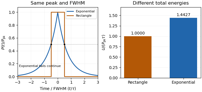
The Gaussian pulse energy and peak power article gives the Gaussian-family relation. Reconstructing an arbitrary pulse's energy requires the full calibrated profile or an additional justified shape model; a width and peak alone cannot supply it.
Nonuniqueness of pulse energy at fixed peak power and FWHM means that those two measurements do not determine the integral of an otherwise unspecified power profile. The pulse energy shape factor gives a rectangular/exponential counterexample. A stronger original construction shows there is no finite universal upper bound without restrictions on lower-level tails.
Fix , power FWHM , and . Choose any . Let the power equal for , equal for , and zero afterward. The optical pulse pedestal is part of the stipulated signal, not an unrelated background. Its level stays below half maximum, so the peak and FWHM remain unchanged, butWith and , the energy is , compared with for the pedestal-free rectangle. Increasing finite gives unbounded pulse energy at fixed peak and FWHM across this family of finite-duration ideal profiles.
This is an identifiability result, not a claim that a particular laser has arbitrarily long tails. The primary source definition of power-FWHM fixes a threshold width, not the integrated energy below that threshold.[ref]
Plane wave and beam source - Simulation object in Ansys Optics documentation. PULSELENGTH definition
A measured full profile, a justified shape family or additional tail-duration bounds supply information that peak and FWHM omit.Unbounded pulse energy at fixed peak and FWHM means there is no universal finite energy upper bound from those two quantities alone. Each pulse can still have finite duration and finite energy. The nonuniqueness of pulse energy at fixed peak power and FWHM article constructs a rectangular core of width and a below-half-maximum pedestal of height extending to total duration .
For any desired energy above the core energy, chooseThis is finite for every finite desired while keeping the peak and power FWHM unchanged. For an original numerical case, take , and . An energy of requires in this ideal profile. The core contributes only .
Additional information changes the problem. If the signal support is bounded by and power outside the FWHM interval is at most , thenThese pulse-energy bounds from tail duration and pedestal height require independently justified tail constraints. A FWHM definition alone fixes a threshold width, not the below-threshold integral.[ref]
Plane wave and beam source - Simulation object in Ansys Optics documentation. PULSELENGTH definition
The construction concerns isolated ideal pulse profiles, not a claim that an actual laser or finite-period pulse train can have arbitrary tails.Pulse-energy bounds from tail duration and pedestal height convert independently justified constraints on low-level light into a bound on total laser pulse energy. Peak power and full width at half maximum alone do not constrain an arbitrarily long below-threshold tail, as unbounded pulse energy at fixed peak and FWHM demonstrates.
Consider a nonnegative isolated power profile with peak , one contiguous half-maximum interval of duration , and total support of duration at most . Suppose power outside that interval is at most . ThenThe lower bound uses the half-maximum condition within the interval. The upper bound fills that interval to and every permitted remaining instant to . These bounds assume the stated shape class; multiple half-maximum crossings require an explicit interval convention.
For an original , , and , they give . Suppose a calibrated measurement additionally determines core energy . The pulse-energy interval from incomplete tail measurements tightens towith the displayed product using watts and nanoseconds. Reducing the independently established tail duration to tightens the upper bound to without changing the measured peak or width.
A receiver with characterized low-level response and a sufficiently long acquisition window is needed to justify and . A trace that falls below a detector threshold establishes no later support cutoff by itself. NIST's pulse-energy calibration discussion separates temporal waveform measurement from background and leakage effects.[ref]
Calibration Service for Low-level Pulsed-Laser Radiometers at 1.06 µm: Pulse Energy and Peak Power by Rodney W. Leonhardt. §§3.4–3.5, transfer and reference standards; §7.2, Leakage Effect
The numerical bounds above are conditional mathematical examples, not specifications of that apparatus.A pulse-energy interval from incomplete tail measurements combines measured energy with bounds on optical power outside the acquisition window. It describes a set of compatible total energies, not automatically a standard uncertainty or confidence interval. The pulse-energy bounds from tail duration and pedestal height article treats a particular peak-and-width model; a window-based construction need not assume that pulse shape.
Suppose true radiant energy inside a measured window lies in a justified interval , with . Partition the unobserved times into regions of durations with independently established nonnegative radiant power caps . ThenFor an original measurement, let the observed-window energy lie between and . An unobserved early region lasting at most contributes at most ; a late region lasting at most contributes at most . The total interval is therefore to . For these assumptions the fraction of optical energy outside a time gate equal to is at most .
A finite support cutoff is sufficient but not necessary for a finite bound. Bounding unobserved optical energy with an exponential tail model uses a validated cap after the window endpoint , which integrates to . Without a justified duration or integrable envelope, one below-threshold reading cannot bound all later energy.
Establish the caps with characterized detector sensitivity, baseline and temporal coverage; do not identify detector ringing directly with optical tails. NIST's response analysis explicitly models the electrical trace as a convolution of the optical waveform with detector response.[ref]
Calibration Service for Low-level Pulsed-Laser Radiometers at 1.06 µm: Pulse Energy and Peak Power by Rodney W. Leonhardt. AppendixC.1, printedp36, impulse response and convolution; AppendixC.2, response-measurement procedure
The interval above follows from chosen optical bounds, not from an uncorrected finite-bandwidth detector trace.A finite optical record can bound later radiant energy if an independently justified exponential decay envelope applies at every later time. Let the recorded window end at , and suppose the true nonnegative radiant power satisfiesIntegration gives the exponential-envelope tail-energy boundEquality holds when the entire tail follows the envelope. This is a bound on an unobserved contribution, not automatically a standard uncertainty or a probabilistic interval.
For an original numerical example, suppose the energy inside the recorded window is known to lie in , while a justified envelope has and . The missing contribution is at most , so the total laser pulse energy lies in . The optical energy outside a time gate fraction, considering only this late contribution, is at most . Any unobserved early energy requires its own bound.
One way to justify the envelope mathematically is a differential inequality for an exponential tail envelope. Suppose is absolutely continuous on each finite interval after , , and almost everywhere. Multiplying by the integrating factor givesso . The decay law must apply throughout the unobserved region; it is a physical assumption to validate, rather than a consequence of fitting the last few samples.
The distinction is testable by a counterexample. Append a later nonnegative pulse whose support lies entirely beyond the recorded interval. Its energy can be arbitrarily large while every recorded sample is unchanged. Such a pulse violates the global envelope but cannot be excluded by a good local exponential fit alone. Similarly, an envelope with a positive constant background has an infinite integral over an infinite time interval. A finite observation horizon or an adequately defined and validated background subtraction is then essential.
Uncertain envelope parameters require a bound valid for their allowed combinations. If the allowed set is the rectangle and , then . For and , this is and the preceding total interval becomes . More restrictive joint parameter constraints can tighten this result; inserting separate best-fit values does not establish a guaranteed bound.
Finally, an electrical tail need not be an optical tail. In an original idealized linear time-invariant system, let a photodetector have unit-area impulse response for , and zero otherwise. An impulsive optical input , with the Dirac delta function, gives the calibrated output by convolution. Its electrical tail after has area even though all incident optical energy arrived at time zero. This optical tail and detector-response ambiguity requires a separate response measurement. NIST's historical procedure characterized the photodetector, cable and oscilloscope together before convolving measured responses with trial waveforms. Appendix C describes typical optical excitation of about , a photodetector rise time near , and a oscilloscope with rise time. The optical excitation was much shorter than the detector response, while the oscilloscope was fast enough that the detector dominated the measured waveform. Response data were collected at each gain setting and several signal levels.[ref]
Calibration Service for Low-level Pulsed-Laser Radiometers at 1.06 µm: Pulse Energy and Peak Power by Rodney W. Leonhardt. Appendix C.1–C.2, printed pp. 36–37
Optical tail and detector-response ambiguity arises because a measured temporal trace combines the optical waveform with the receiver's dynamics. In a calibrated linear time-invariant system,where is incident radiant power and the unit-area detector impulse response. One trace does not generally identify both unknown functions. The parent bounding unobserved optical energy with an exponential tail model gives an impulsive-input example; two finite-width profiles provide another exact ambiguity.
Define for , and zero otherwise. Consider model A with optical power and detector response , and model B with these two time constants exchanged. By commutativity of convolution, both give exactlyTheir optical energies after are nevertheless and . For original chosen , those are about and . Identical recorded tails therefore coexist with very different true late optical energy.
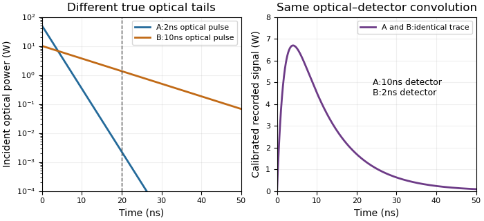
Different optical tails and detector responses can produce the same measured pulse
. Original unit-area exponential response models. Model A has a2ns optical time constant and10ns detector time constant; model B exchanges them. Both incident pulses have100nJ total energy. The measured convolution is identical despite different optical energy after20ns. Source. Details.Known-input calibration of a pulse detector supplies information missing from this inverse problem. NIST measured the detector/cable/oscilloscope response with optical excitation much shorter than the response before calculating waveform distortions.[ref]
Calibration Service for Low-level Pulsed-Laser Radiometers at 1.06 µm: Pulse Energy and Peak Power by Rodney W. Leonhardt. Appendix C.1–C.2, printed pp. 36–37, Figure C1 and bandwidth-correction procedure
The example above is an independent mathematical construction. A fitted electrical decay constant alone cannot establish a global optical-tail envelope.Known-input calibration of a pulse detector uses a characterized optical waveform to separate the incident signal from the receiver response. In a linear, baseline-corrected model,where is known input power, a normalized impulse response and the overall responsivity. Recording the complete response givesThus a known reference energy calibrates the area gain without requiring the input to be an ideal impulse. Shape calibration additionally uses the reference waveform.
For nonnegative normalized profiles with finite second moments, define and . Since , their temporal variances satisfy . In an original chosen example, an input standard deviation and recorded deviation imply . Treating that finite input as a delta impulse would incorrectly assign the full to the detector. This finite-input correction in pulse-detector calibration concerns standard deviations; a universal subtraction rule for arbitrary FWHM values does not follow. Negative ringing also invalidates the nonnegative-profile interpretation used for the variance identity.
NIST's primary procedure illuminated the detector with a pulse much shorter than the detector response and characterized detector, cable and oscilloscope together at the relevant gain and signal levels.[ref]
Calibration Service for Low-level Pulsed-Laser Radiometers at 1.06 µm: Pulse Energy and Peak Power by Rodney W. Leonhardt. §§6.1–6.2; Appendix C.1–C.2, printed pp. 36–37, Figure C1 and measurement procedure
Such a known input breaks the optical tail and detector-response ambiguity described by the parent article.In the frequency domain, the same model is . Division can estimate where the input spectrum is known and sufficiently nonzero; small input components amplify measurement noise. A short reference pulse is useful because it excites a broad frequency range, but detector linearity, baseline, area coverage and reference uncertainty still need checking.
Finite-input correction in pulse-detector calibration removes the known input duration from an inferred receiver width, while propagating uncertainty in both widths. Under the nonnegative, normalized, finite-variance convolution model of known-input calibration of a pulse detector,where is the known input profile, the measured output and the receiver's impulse response. The subtraction concerns temporal variances, not arbitrary reported full widths.
Differentiating on the positive-width branch givesFirst-order propagation of standard uncertainty therefore yieldsThe covariance matters when both widths use the same timebase or fitted reference.[ref]
An original near-resolution example has and , each with independent standard uncertainty . The corrected receiver width is and its propagated standard uncertainty is about , or . Width measurements individually precise to about one percent can thus give a much less precise difference-derived width.
NIST's primary bandwidth-correction procedure used roughly 120 ps optical inputs and recorded the detector, cable and oscilloscope as one response chain at different gains and signal levels.[ref]
Calibration Service for Low-level Pulsed-Laser Radiometers at 1.06 µm: Pulse Energy and Peak Power by Rodney W. Leonhardt. Appendix C.1–C.2, printed pp. 36–37, Figure C1 and steps 1–7
A sufficiently short characterized input reduces this resolution-limit conditioning in finite-input detector calibration. Near a zero variance difference, linear uncertainty propagation may fail; a nonpositive measured difference does not represent a negative physical detector width. Report an interval or limit under the stated model rather than silently replacing the difference by zero. Negative ringing also violates the nonnegative-profile assumption behind the variance subtraction.Resolution-limit conditioning in finite-input detector calibration is the sensitivity of a small inferred detector width to uncertainty in two nearly equal measured widths. In finite-input correction in pulse-detector calibration, the nonnegative normalized convolution model givesThe signed relative sensitivities areThey diverge as the measured output width approaches the known input width . Subtracting two well-measured squared widths can therefore be a poorly conditioned inference.
For an original example, and give and . The two relative sensitivity coefficients are about and . A small independent fractional width error can produce a much larger fractional response-width error; a common multiplicative timebase error instead partly cancels because the coefficients sum to one. Correlations must therefore be retained.[ref]
Near the boundary, report uncertainty in the variance difference before transforming it. For a chosen interval , imposing the physical constraint gives a detector-width interval , approximately . A coverage-preserving detector-width bound from a variance interval uses this monotone square-root transformation on the physical intersection. It need not resemble a symmetric error bar around a point estimate. An interval wholly below zero contains no admissible width under this model; replacing it silently with a zero-width result hides the inconsistency.
NIST characterized its detector/cable/oscilloscope chain with an optical pulse much shorter than the receiver response.[ref]
Calibration Service for Low-level Pulsed-Laser Radiometers at 1.06 µm: Pulse Energy and Peak Power by Rodney W. Leonhardt. Appendix C.1–C.2, printed pp. 36–37; approximately 120 ps optical input and Figure C1
That design avoids subtracting two nearly equal broad widths. The variance identity still requires nonnegative profiles and finite second moments; arbitrary full widths at half maximum and responses with negative ringing need a different model.A coverage-preserving detector-width bound from a variance interval transforms uncertainty in a nonnegative response variance without imposing a symmetric width error bar. Let and let a random interval have stated frequentist coverage for . Define the width confidence set byFor the true width ,The events are identical, so their coverage probabilities are identical. The transformation does not create coverage that the original interval lacked. Resolution-limit conditioning in finite-input detector calibration explains why working with the variance difference first is useful near a barely resolved detector response.
For an original explicit measurement model, suppose has a normal distribution with mean and known standard deviation . A reading gives an approximately 95 percent interval . Intersecting with the physical range and taking square roots gives . This is an assumed normal model for measuring , not a claim that any difference of fitted squared widths is automatically normal.
If the entire variance interval is negative, the result is an empty physical confidence set for a detector variance difference. Do not replace its negative upper endpoint by zero and report an apparently exact zero width: that changes the confidence-set construction. An empty realization signals disagreement between that interval and the physical parameter range; it can occur even in a valid procedure on an occasional sample that misses the true value.
NIST distinguishes a standard uncertainty from an interval with a justified confidence level and explains the distributional assumptions behind a coverage factor near two.[ref]
Guidelines for Evaluating and Expressing the Uncertainty of NIST Measurement Results by Barry N. Taylor and Chris E. Kuyatt. §§6.2–6.3, Expanded Uncertainty
The normal interval above needs its stated model; the monotone transformation proof itself does not. Application to a detector additionally requires the nonnegative-profile convolution assumptions of finite-input correction in pulse-detector calibration; a correct statistical transformation cannot repair an invalid physical variance identity.An empty physical confidence set for a detector variance difference occurs when the entire reported interval for the inferred response variance lies below its admissible range. In the nonnegative-profile detector model, . An interval gives a physical width setIt is empty exactly when . The coverage-preserving detector-width bound from a variance interval proves why this intersection and transformation retain the original coverage event.
For an original reading, suppose an explicitly normal measurement model for gives with known standard deviation . The approximately 95 percent interval contains no nonnegative variance. This is disagreement between that interval and the physical model, not a negative physical detector width or an exact measurement of zero width.
Empty sets can occur occasionally even when the model is correct. If and , thenwhere is the standard normal cumulative distribution function. At the physical boundary and , the probability is about ; at it is about . The boundary probability of an empty detector-width confidence set explains why one empty realization is not a logical disproof of the detector model.
Replacing an empty set by the point zero changes the procedure. It must not be presented as though the original interval precisely determined that point. NIST likewise distinguishes an uncertainty interval from an automatically justified confidence level, emphasizing the distributional assumptions behind coverage factors.[ref]
In practice, examine the width estimates, their correlations and the physical convolution assumptions, while retaining the actual negative interval in the measurement record. NIST's short-input receiver-response measurement illustrates how an independently characterized input helps resolve detector broadening.[ref]
Calibration Service for Low-level Pulsed-Laser Radiometers at 1.06 µm: Pulse Energy and Peak Power by Rodney W. Leonhardt. Appendix C.1–C.2, printed pp. 36–37, Figure C1
Neither clipping the estimate nor declaring the response model false follows solely from the sign of one noisy variance difference.The boundary probability of an empty detector-width confidence set is the chance that a valid uncertainty procedure yields no admissible nonnegative response width when the true variance difference is at its boundary. Under the explicit model , , take the central interval . The empty physical confidence set for a detector variance difference occurs when its upper endpoint is negative:This probability decreases with , so the largest value over the physical parameter range occurs at . If is the usual two-sided normal critical value, the boundary probability is .
At that boundary the other way to miss zero is a strictly positive lower endpoint. The two tail events are disjoint and each has probability ; the remaining probability produces a confidence set containing zero. The joint probability of empty and strictly positive detector-width intervals therefore accounts for the full two-sided noncoverage, not just the empty cases.
For an original repeated-measurement calculation, use and 400 independent measurements of a stipulated zero response-variance difference. The expected number of empty physical sets is approximately ten, with standard deviation , where . The count follows a binomial distribution only under the stated independent, common-probability model. Roughly ten additional intervals are expected to lie wholly above zero. Their existence is compatible with approximately 95 percent coverage at the boundary.
For an interior example , the empty-set probability falls to . Empty results are thus most common near the resolution boundary, where subtracting similar measured variances is already delicate.
NIST explains that interpreting expanded uncertainty as a confidence interval requires distributional assumptions.[ref]
Guidelines for Evaluating and Expressing the Uncertainty of NIST Measurement Results by Barry N. Taylor and Chris E. Kuyatt. §§6.2–6.3, Expanded Uncertainty
These probabilities assume an actual normal model with known ; they are not inferred merely from an error bar labelled standard uncertainty. Correlation, systematic offsets or a misspecified detector response can change the repeated-measurement behavior. Retaining empty results in the record allows that behavior to be assessed rather than hiding it by replacing them with zero-width estimates.The joint probability of empty and strictly positive detector-width intervals must distinguish outcomes of one measurement from counts across repeated measurements. For one normal variance-difference estimate , let . An empty physical width set requires ; a strictly positive interval requires . Those events are disjoint for that same interval, so their intersection has probability zero.
Writing and for the standard normal cumulative distribution function, the three category probabilities areThe last category is an interval containing zero. At and a central interval, these become , as in boundary probability of an empty detector-width confidence set. For interior , the categories describe the relation to zero; they are not themselves the coverage categories for the true positive value.
For independent repetitions with the same probabilities, the counts have a multinomial distribution. For nonnegative integers summing to ,Although the measurement repetitions are independent, their category counts are not. An empty and a positive indicator cannot both equal one in the same repetition, givingThis negative covariance of empty and positive detector-interval counts follows from the fixed total count.
For an original example, take 20 independent boundary measurements with exact central 95 percent normal intervals. Then . Each count has mean , and their covariance is . The probability of exactly one empty and one strictly positive interval is , about . It is not zero, unlike the intersection of those two outcomes for a single interval.
NIST's uncertainty guidance emphasizes the assumptions needed to assign confidence levels.[ref]
Guidelines for Evaluating and Expressing the Uncertainty of NIST Measurement Results by Barry N. Taylor and Chris E. Kuyatt. §§6.2–6.3, Expanded Uncertainty
The joint-count calculation above additionally assumes independent repetitions with a common normal model; shared calibration errors can invalidate that independence even when each marginal interval is computed in the same way.The negative covariance of empty and positive detector-interval counts arises because a fixed number of measurement intervals is divided into mutually exclusive categories. Let indicate that interval is respectively physically empty or strictly positive. The same interval cannot satisfy both, so andFor independent repetitions with common probabilities, the counts and therefore haveThe joint probability of empty and strictly positive detector-width intervals gives the underlying multinomial model. The sign describes category-count dependence, not physical antagonism between two detectors.
For an original boundary example, take and . Each count has variance , while their covariance is . The total tail-category count has variance . Treating the two counts as independent would give instead. The covariance is needed even though the individual measurement repetitions are independent.
Conditioning on the total is important. If the number of repetitions is random and independent of the category assignments, the law of total covariance givesAn independent total with a Poisson distribution has equal mean and variance, making this covariance zero; a more variable total can make it positive. This is a different sampling protocol, not a contradiction of the fixed-total formula.
Shared calibration drift is another change of model. Repetitions may then have dependent category indicators, and cross-repetition covariance terms must be added. Overdispersion of detector-interval counts under shared drift can make a simple multinomial analysis inadequate.
NIST's measurement guidance retains common influences in uncertainty propagation and requires assumptions for confidence-level interpretation.[ref]
Guidelines for Evaluating and Expressing the Uncertainty of NIST Measurement Results by Barry N. Taylor and Chris E. Kuyatt. Appendix A, equation A-3; §§6.2–6.3, Expanded Uncertainty
State whether the repetition total is fixed, how the categories are defined and which calibration influences are shared before interpreting their empirical count covariance.Effective repetition count across independent calibration blocks accounts for dependence confined to each acquisition block rather than shared by every stored trace. Suppose block contains empty-interval indicator random variables, all with common probability and within-block correlation coefficient . Assume different blocks are independent. With , summing within-block covariances givesMatching this to the variance of an average of independent indicators yieldsFor equal blocks of size , this reduces to . The denominator involves the block size, not the total ; the single-block expression in effective repetition count for detector intervals with shared drift must not be applied as though the same drift state affected every block.
For an original comparison, fix and . One block gives . Six independent blocks of twenty give . Six very uneven blocks of sizes instead giveAll three designs store the same number of traces. The difference comes from how often the same fluctuating condition is reused. For fixed , , and positive , minimizing favors balanced blocks; this motivates optimal allocation of detector repetitions across calibration blocks when block-preparation costs also matter.
Independence must come from the physical acquisition model. Starting another file does not erase a shared clock, reference calibration, or slowly varying environmental influence. NIST's uncertainty law retains shared-input covariance explicitly.[ref]
Guidelines for Evaluating and Expressing the Uncertainty of NIST Measurement Results by Barry N. Taylor and Chris E. Kuyatt. Appendix A, equation A-3
If drift persists between nominal blocks, those cross-block terms must be added and the displayed formula changes. A cluster bootstrap likewise requires blocks that are suitable independent resampling units.Optimal allocation of detector repetitions across calibration blocks chooses block sizes using the dependence and acquisition-cost model, not just the desired number of stored traces. For fixed total , number of independent blocks , common success probability, and positive within-block correlation , effective repetition count across independent calibration blocks givesMaximizing it is equivalent to minimizing . If two integer block sizes differ by at least two, transferring one repetition from the larger to the smaller decreases that sum by . Therefore the optimal integer sizes differ by at most one.
For an original fixed-count example, and give balanced sizes . At , their effective count is . Sizes give only under the same assumptions.
More independent blocks can help, but preparing one may consume time. In a continuous planning model let each block cost setup time , each repetition cost , and each block contain repetitions. With total time , the effective count becomesFor , differentiation gives the interior choice . Integer block counts, minimum sizes, and hardware restrictions must subsequently be imposed.
For chosen , , and , the continuous optimum is feasible with ten blocks and gives . Single-repetition blocks give 18, while two blocks of 81 repetitions also give 18. These are model-based comparisons, not measured apparatus timings.
Unequal block noise or different drift correlations require unequal-noise allocation across calibration blocks. Independence between prepared blocks must also be justified by the reference and environmental model; NIST explicitly retains shared-input covariance.[ref]
Unequal-noise allocation across calibration blocks distributes repetitions using block-specific variability while keeping the intended estimator fixed. Suppose independent blocks supply means and the target estimate is with specified weights . Let one observation in block have variance and equicorrelation within that block. ThenThe first sum is a block-specific floor; only the second decreases with repetition count. Changing the estimator weights merely to improve this calculation could change the estimand, so they remain fixed here.
For continuous positive allocations with positive costs , budget and , a Lagrange-multiplier calculation givesFor equal observation costs, repetitions are proportional to , not to the variance itself. Minimum counts and integer rounding must subsequently respect the actual acquisition constraints.
For an original two-block example, take , equal costs, , independent readings within each block, and standard deviations and in the output unit. The optimal counts are and , giving variance instead of from fifty each. If both within-block correlations are instead , the same proportions give variance , while equal counts give . The common-error floor now dominates and cannot be eliminated by taking more observations inside those same blocks.
This extends optimal allocation of detector repetitions across calibration blocks, whose balanced solution used homogeneous noise. For binary detector indicators, the per-reading variance is ; differing probabilities require a clearly specified weighted target. The planning variances and correlations must come from an appropriate measurement calibration model, not merely from counting files as independent blocks. NIST's uncertainty propagation retains shared-input covariance for exactly this reason.[ref]
An exponential-envelope tail-energy bound limits unobserved energy by integrating a justified pointwise envelope on the true optical power. If for every , with and , then . The parent bounding unobserved optical energy with an exponential tail model derives this result and distinguishes it from a statistical uncertainty.
At a later acquisition endpoint , the remaining allowance isFor an original envelope with and , the initial allowance is . Reducing the allowed missing energy to requires . This acquisition duration from an exponential tail-energy tolerance reduces the bound by a factor100. It does not prove that99% of an arbitrary underlying pulse has been captured: the actual power may lie strictly below the envelope at early times.
Joint parameter constraints also matter. An original allowed set uses dimensionless and with , and . Since , every allowed envelope satisfiesattained at . Taking separate maxima and would instead give the looser bound; those two maxima cannot occur together in the stated joint set.
The guarantee concerns optical power, not an uncorrected detector tail. Optical tail and detector-response ambiguity explains that distinction, while NIST's primary response-calibration procedure characterizes the electrical measurement chain separately.[ref]
Calibration Service for Low-level Pulsed-Laser Radiometers at 1.06 µm: Pulse Energy and Peak Power by Rodney W. Leonhardt. Appendix C.1–C.2, printed pp. 36–37
A delayed extra pulse or an unbounded constant background requires its own model; neither is excluded by a local exponential fit.An acquisition duration from an exponential tail-energy tolerance chooses how long to continue recording when a validated optical-power envelope bounds the remaining energy. Suppose after time the true power satisfies , with and . The exponential-envelope tail-energy bound gives a remaining allowance after extension . For tolerance ,This is a conditional upper-bound calculation, not an inference from the last sample merely falling below a detector threshold.
An original uncertainty example has guaranteed parameter limits and . The remaining allowance increases with either parameter, so a tolerance requires . Using only best-fit values and would give about , which does not guarantee the same tolerance over the allowed set. Joint parameter constraints can tighten a bound, but their coverage must be justified.
In the positive-duration branch, the local sensitivities areThis acquisition-time sensitivity to tail-model parameters explains why an uncertain slow decay can matter more than a small amplitude correction. The derivatives change interpretation at the zero-duration boundary.
The envelope must apply to optical power throughout the unrecorded region. A later pulse or an unremoved persistent background can invalidate it. NIST's separate measurement of detector response illustrates why an electrical waveform's decay alone is insufficient.[ref]
Calibration Service for Low-level Pulsed-Laser Radiometers at 1.06 µm: Pulse Energy and Peak Power by Rodney W. Leonhardt. Appendix C.1–C.2, printed pp. 36–37
State the chosen time origin, tolerance units, valid envelope parameters and any other excluded intervals when reporting the acquisition requirement.Acquisition-time sensitivity to tail-model parameters measures how an inferred recording extension changes when the assumed optical tail changes. In the positive-duration branch of acquisition duration from an exponential tail-energy tolerance, writeHere bounds the initial tail power, is its decay time and the tolerated missed energy. Their first-order relative effects areThese logarithmic condition numbers of a tail-acquisition requirement distinguish a fractional amplitude error from a fractional decay-time error. For a stringent tolerance with large , decay-time sensitivity stays near unity while amplitude sensitivity decreases.
For an original example, take , and . Then and . Let the independent standard uncertainties of and be and , with the tolerance fixed. The amplitude contribution to is ; the decay-time contribution is . Adding their variances gives , about .
Correlated fitted parameters require covariance terms in this propagation.[ref]
Guidelines for Evaluating and Expressing the Uncertainty of NIST Measurement Results by Barry N. Taylor and Chris E. Kuyatt. Appendix A, equation A-3
A standard uncertainty is not a guaranteed recording margin: a worst-case requirement needs a justified allowed parameter set, as in the parent article. The zero-duration boundary is also outside this smooth positive-branch calculation.Physically, these parameters must describe the unrecorded optical power, not merely an electrical detector tail. NIST separately measured the detector/cable/oscilloscope response before correcting pulse measurements.[ref]
Calibration Service for Low-level Pulsed-Laser Radiometers at 1.06 µm: Pulse Energy and Peak Power by Rodney W. Leonhardt. Appendix C.1–C.2, printed pp. 36–37
A precise fit to the wrong response component does not justify the optical envelope or its acquisition-time bound.Logarithmic condition numbers of a tail-acquisition requirement quantify the fractional response of a positive recording extension to fractional parameter changes. For with , define the signed sensitivity . ThenTheir absolute values are componentwise relative condition numbers. Acquisition-time sensitivity to tail-model parameters gives the corresponding dimensional derivatives and uncertainty propagation.
These numbers depend on which coordinates are held fixed. If denotes the initial tail-energy allowance, then . In coordinates , the decay-time sensitivity at fixed is exactly one, rather than . This is the same physical formula: holding fixed while changing also changes . Transforming the parameter covariance consistently leaves the propagated output uncertainty unchanged.[ref]
An original boundary example takes and . The required extension is only , but . Increasing by multiplies the ratio by , giving and doubling the required extension exactly. Its relative change is large because the original extension was very small.
This does not mean the absolute requirement is singular there. In the active branch remains finite. At and below the threshold, the physical extension is zero, so is undefined. A logarithmic tail-duration change at the zero-extension boundary must instead use the piecewise requirement or absolute changes. Large relative conditioning alone is not evidence of a large absolute recording-time risk.
Finally, conditioning describes the stated envelope model, not its experimental validity. The optical power tail must be distinguished from detector response, which NIST measured independently in its pulse calibration procedure.[ref]
Calibration Service for Low-level Pulsed-Laser Radiometers at 1.06 µm: Pulse Energy and Peak Power by Rodney W. Leonhardt. Appendix C.1–C.2, printed pp. 36–37
A well-conditioned calculation based on an invalid optical envelope still gives an unjustified acquisition guarantee.Logarithmic tail-duration change at the zero-extension boundary describes a recording requirement whose input ratio crosses the point where no further acquisition is needed. For fixed decay time , put and . The physical extension isHere the logarithm applies to the input ratio, not to a zero output duration. Logarithmic condition numbers of a tail-acquisition requirement applies only where .
At , the left derivative is zero and the right derivative is . The directional derivative of a clipped logarithmic acquisition time along a signed input change isThus no single ordinary derivative describes threshold-crossing perturbations. Nevertheless, the duration is stable in absolute units:This follows because the positive-part map has Lipschitz continuity with constant one.
For an original interval example, take and a justified input-ratio range . The corresponding duration range is . Its lower part is clipped at zero. Linearizing only on the zero-duration side would incorrectly predict no possible extension even though the allowed set crosses the threshold. A relative error divided by a nominal is undefined, while this absolute bound remains meaningful.
If is uncertain too, optimize the full expression over the justified joint parameter set rather than treating this fixed- inequality as a complete uncertainty analysis. The tail model must bound optical power throughout the missed interval. NIST's calibration apparatus measured detector/cable/oscilloscope response separately, illustrating why a recorded electrical decay cannot automatically certify such an optical envelope.[ref]
Calibration Service for Low-level Pulsed-Laser Radiometers at 1.06 µm: Pulse Energy and Peak Power by Rodney W. Leonhardt. Appendix C.1–C.2, printed pp. 36–37
The clipping analysis is an original property of the stated conditional acquisition model.The directional derivative of a clipped logarithmic acquisition time describes the first-order recording extension when several envelope parameters change together at the acquisition threshold. For positive , writeThe logarithmic tail-duration change at the zero-extension boundary article treats a fixed decay time and logarithmic input coordinate. Here consider a boundary point and an additive parameter direction .
The one-sided directional derivative uses positive step sizes:The logarithmic chain rule gives the expression inside the maximum. Differentiating the prefactor contributes zero at the boundary because the clipped logarithm there is zero.
For an original example, let , and . Increase amplitude in direction while decreasing decay time in direction , with . The net fractional direction is , so per unit step. Reversing the direction gives derivative zero, not .
The derivative is positively homogeneous in the direction but is not linear, so no single gradient represents all threshold-crossing perturbations. Above threshold the usual smooth derivative applies; strictly below threshold all sufficiently small changes leave the extension zero. Gaussian input uncertainty at a clipped acquisition-time threshold can consequently produce a mass of outcomes exactly at zero rather than a symmetric distribution around a nominal duration. The directional calculation alone does not assign a confidence level.
This is a conditional optical-envelope calculation. Separating optical power from the receiver's electrical response remains necessary before its parameters describe missed light. NIST independently characterized the detector/cable/oscilloscope response in its pulse calibration procedure.[ref]
Calibration Service for Low-level Pulsed-Laser Radiometers at 1.06 µm: Pulse Energy and Peak Power by Rodney W. Leonhardt. Appendix C.1–C.2, printed pp. 36–37
A derivative can describe parameter sensitivity accurately while the envelope itself still needs experimental justification.Gaussian input uncertainty at a clipped acquisition-time threshold produces a mixed output distribution rather than an ordinary Gaussian error bar. Hold the decay time fixed and assume the logarithmic input ratio has distribution , with . The required extension isThe directional derivative of a clipped logarithmic acquisition time explains the kink; here the full input distribution is propagated through it.
Writing and for the standard normal cumulative distribution function and density, respectively,For the continuous part has density . It integrates to less than one because the remaining probability is an atom at zero. Treating this density alone as the entire distribution loses that atom.
At the nominal threshold , half the outcomes are zero and the conditional positive part has a half-normal distribution. Direct integration of the normal density givesFor an original example, and logarithmic standard deviation give mean extension about and standard deviation , although inserting the nominal input into the clipped formula gives zero. The probability of an extension above is .
The quantiles of a clipped Gaussian acquisition duration must likewise include the zero atom. A symmetric interval around the nominal zero duration cannot represent these probabilities. NIST's uncertainty discussion stresses the need to know and combine input distributions when assigning an interval probability.[ref]
This is a stated uncertainty model for a conditional recording requirement, not a worst-case optical-energy guarantee. Uncertain decay time, correlation among the original envelope parameters or a non-Gaussian logarithmic ratio requires the corresponding joint propagation instead. Establishing the optical envelope remains a separate experimental task.
Quantiles of a clipped Gaussian acquisition duration assign probability levels to a recording extension whose distribution has a point mass at zero. Under the model of Gaussian input uncertainty at a clipped acquisition-time threshold, let , , and for fixed . Its zero mass is .
Using the lower generalized quantile for givesEquivalently, . The constant branch is essential: directly using a negative untruncated normal quantile would assign an impossible negative duration. SciPy's normal-distribution documentation identifies
ppf as the inverse cumulative distribution function used for the Gaussian part of this calculation.[ref]For an original threshold example, take , and . Half the probability is at zero, so the median is zero. The 90th and 95th percentiles are approximately and . The one-sided interval has probability under this stated model.
A nominal equal-tail 95 percent construction behaves differently: actually contains probability . Its lower endpoint includes the entire zero atom instead of excluding a 2.5 percent lower tail. This coverage excess from central quantiles at a zero-duration atom is a property of the mixed distribution, not a rounding error.
Quantiles describe uncertainty in the conditional acquisition requirement. They are not automatically a frequentist confidence set for an unknown fixed physical duration, nor a worst-case guarantee on unrecorded optical energy. NIST explains why an interval's probability interpretation requires the underlying distributions and assumptions.[ref]
Guidelines for Evaluating and Expressing the Uncertainty of NIST Measurement Results by Barry N. Taylor and Chris E. Kuyatt. §6.3, Expanded Uncertainty
Propagate any uncertainty in decay time or other envelope parameters jointly before applying this fixed- formula.Coverage excess from central quantiles at a zero-duration atom is the additional distributional probability included when a closed quantile interval captures an entire point mass at zero. Here coverage means probability under the stated duration model. For with , the zero mass is and the positive part is continuous. Let , , and use the lower quantiles from quantiles of a clipped Gaussian acquisition duration.
For the closed central interval , its probability isTo verify this, write the probability as . When both endpoints are positive, the lower left limit is and the upper value is . Once the lower endpoint is zero, its left limit is zero; if the upper endpoint is zero too, the interval contains exactly the zero atom. Endpoint inclusion is therefore part of the probability calculation.
For a nominal 95 percent central construction, zero masses , and give actual probabilities , and respectively. In the middle case, the excess is , not the whole atom: the interval already includes the probability between zero and the upper quantile.
As an original dimensional example, set , and , giving . The nominal central 95 percent interval is approximately and contains probability . SciPy documents the normal cdf and inverse-cdf ppf used to evaluate these Gaussian-component values.[ref]
SciPy 1.16.2 documentation. scipy.stats.norm, Methods: cdf and ppf
A one-sided upper interval or a separately specified probability construction can target a different included probability. Randomized endpoint inclusion at a zero-duration atom would require an explicit randomization rule, not a change made silently after seeing an endpoint equal zero. NIST explains why interval interpretation requires the input distributions and the chosen construction.[ref]
Guidelines for Evaluating and Expressing the Uncertainty of NIST Measurement Results by Barry N. Taylor and Chris E. Kuyatt. §6.3, Expanded Uncertainty
Distributional probability for this conditional acquisition model is separate from a worst-case optical-energy guarantee or a confidence procedure for an unknown fixed parameter.Randomized endpoint inclusion at a zero-duration atom adds an independent random decision about whether an interval contains the atom, allowing an exact included probability under a specified distribution. Let the duration have zero mass and a continuous positive part. For a nominal central level , put , and assume . Choose upper endpoint with .
The coverage excess from central quantiles at a zero-duration atom shows that the closed set has probability , while has probability . Draw an independent and reportThen the joint probability over both and the auxiliary random draw isThe independence assumption is essential to the multiplication .
For an original example, let and . The endpoint is included with probability . The positive part contributes probability and randomized zero inclusion contributes , totaling . An individual reported set is still either closed, with duration-model probability , or open at zero, with probability . Exact applies to the randomized procedure jointly, not conditionally to each realized set.
The distribution sensitivity of randomized zero-endpoint probabilities matters if or the upper endpoint is estimated inaccurately. Plugging a guessed atom probability into does not establish the same equality for the true distribution. The pinned numerical reference documents a standard uniform distribution and its random-variates method, while its normal cdf/ppf methods evaluate the Gaussian component when the duration comes from a clipped normal input.[ref]
This is a mathematical probability construction. It does not remove the atom physically, improve measurement precision, or create a worst-case guarantee on missed optical energy. Its randomization rule and probability interpretation must be specified as part of the procedure.
Distribution sensitivity of randomized zero-endpoint probabilities quantifies how the probability equality in randomized endpoint inclusion at a zero-duration atom changes when its assumed duration law is wrong. Let the nominal law have zero-atom probability , choose a positive upper endpoint with nominal cumulative distribution function , and put , with . Use the parent's independently randomized decision to include zero.
If the actual zero probability is and the actual cumulative distribution function is , the included probability isSubtracting the target separates the two model errors:The first term is upper-endpoint probability error; the second is atom-probability error in a randomized endpoint rule. This identity is an algebraic consequence of independence of the auxiliary random draw, not a normal-approximation result. The documented uniform distribution random-variates construction supplies that auxiliary draw; normal cdf/ppf routines can evaluate a specified clipped-normal duration model.[ref]
For an original misspecification example, choose , , and , so . Suppose instead and . Thenwhich is below : comes from the upper endpoint and from the atom. These are stipulated distributions, not measured failure rates.
More generally, bounds and imply . This propagates validated model-error bounds only. Estimating the nominal law from the same observation used for the interval can add dependence; the unconditional fixed-rule identity then requires an appropriate joint or conditional argument.
Atom-probability error in a randomized endpoint rule is the change in included duration-model probability caused by using an inaccurate zero-atom probability in the randomization. Let , and hold the positive upper endpoint fixed at an actual cumulative distribution function value . If the true zero probability is but the rule uses a positive , its independent endpoint-inclusion probability is . Conditional on that chosen value,This is the atom term isolated in distribution sensitivity of randomized zero-endpoint probabilities, with upper-endpoint error deliberately removed. Underestimating reduces inclusion; overestimating it increases inclusion. The independent auxiliary draw can be generated from a uniform distribution.[ref]
SciPy 1.16.2 documentation. scipy.stats.uniform, support and rvs
If comes from an independent calibration, conditional probabilities must also be averaged over that calibration. For an original example, take , , and . Suppose the calibration returns or with equal probability. Its estimate is unbiased, yet the resulting included probabilities are and , averaging about rather than .
More generally, for an unbiased positive estimate in the valid rule range, Jensen's inequality givesThis reciprocal-estimation bias in randomized atom inclusion comes from a nonlinear plug-in rule, even with independent calibration. It does not identify the size of the error without a calibration model. Values below , including zero, require an explicitly defined clipped or guarded rule; the displayed inverse formula cannot simply be used there.
If a validated upper bound is available and , choosing instead guarantees under the fixed-upper-endpoint and independence assumptions. It may be conservative rather than exact. Uncertainty in remains a separate error term, and these are probabilities for a duration distribution, not a removal of the physical zero-duration atom.
Reciprocal-estimation bias in randomized atom inclusion quantifies the nonlinear plug-in loss beyond the sign supplied by Jensen's inequality. Keep the independent-calibration model of atom-probability error in a randomized endpoint rule: true atom probability , unbiased estimate , and included probability , with the upper endpoint calibrated to actual probability . Assume , , and .
The exact algebraic identitygivesThus the loss depends on squared errors weighted by the reciprocal estimated probability. The second-order delta method approximation is , but the exact remainder shows why small estimated probabilities deserve particular attention.
If almost surely for , a nonasymptotic bound isFor an original small-error example, let , let measurement calibration return or equally often, and take , . Here and the variance is . The exact included probability is about ; the second-order approximation is , while the bounded-error calculation puts the coverage loss between about and .
The bounded-relative-error assumption can fail for a finite binomial measurement calibration: an empirical atom fraction can be zero with positive probability. Such near-zero probability estimates in reciprocal plug-in rules require an explicitly defined guard or different measurement calibration model, not division by zero. The auxiliary endpoint decision must remain independent of the future duration and measurement calibration as stipulated. The documented uniform random-variates construction supplies that auxiliary randomness; it does not validate the atom estimate.[ref]
SciPy 1.16.2 documentation. scipy.stats.uniform, support and rvs
Near-zero probability estimates in reciprocal plug-in rules can make a nominal randomization undefined even when the underlying probability estimate is unbiased. For an independent measurement calibration count , the empirical atom fraction has , butThus its reciprocal is not a finite statistic on every measurement calibration outcome. The binomial probability mass function supplies this zero-count probability directly.[ref]
SciPy 1.16.2 documentation. scipy.stats.binom, Notes: pmf; Methods: pmf
In reciprocal-estimation bias in randomized atom inclusion, a fixed upper endpoint contributes actual probability and the auxiliary rule uses . Valid probabilities require a separate rule when , including zero. One possible numerical guard is with . It makes defined and between zero and one. It does not preserve the unbiasedness or the coverage properties of the unguarded formula.
For an original finite measurement calibration example, take , , , , and . A zero count occurs with probability about . On that outcome the guarded rule includes zero with probability , and its included duration-model probability is , below the nominal . Averaging over every measurement calibration outcome givesThe calculation assumes the future duration, measurement calibration sample, and auxiliary random draw have the stipulated independence, and the upper-endpoint probability is exactly .
Such finite-calibration guards for reciprocal endpoint randomization solve a domain problem, not a coverage proof. A validated upper probability bound can provide a different conservative construction under the parent's assumptions, but an arbitrary floor is not automatically such a bound. Calibration size, lower-tail events and the actual guarded rule must all enter the final joint-probability calculation.
Finite-calibration guards for reciprocal endpoint randomization must specify both a valid endpoint decision and how calibration uncertainty enters its probability guarantee. An arbitrary positive floor avoids division by zero but does not establish nominal inclusion, as the example in near-zero probability estimates in reciprocal plug-in rules demonstrates.
One finite-sample construction uses an upper confidence bound for the atom probability , based on independent calibration count . Supposewhere is a calibration failure budget. An exact one-sided binomial bound can be obtained by inversion: for , choose satisfying , and put . This is a confidence statement over calibration samples, not a posterior probability for a fixed after observing one count. The pinned reference documents the exact binomial proportion-interval method.[ref]
SciPy 1.16.2 documentation. BinomTestResult.proportion_ci, confidence_level, exact method and returned bounds
For a fixed upper duration endpoint with actual cumulative probability , setThe rule is defined and . On the event , its conditional included probability is . This calculation also requires independence of the calibration, future duration and auxiliary endpoint draw as stipulated by the parent model.
For an original zero-count example, take and . Since , inversion gives . With , , and stipulated true , the zero-count conditional included probability is approximately . The bound is much larger than the raw estimate zero, reflecting the uncertainty of a small calibration sample rather than inventing a measured atom fraction.
The calibration confidence level is not free. Since included probabilities are nonnegative even on the failure event, a general joint guarantee from this argument is onlyAt conditional target and calibration confidence , this lower guarantee is , not . To certify an unconditional target using this argument, the conditional target must be at least , provided it can fit below , or the failure budget must be reduced. Any upper-endpoint model error also needs separate accounting.
A differential inequality for an exponential tail envelope supplies a sufficient decay condition for a global power bound. Let nonnegative be absolutely continuous on every finite interval after , with andalmost everywhere, for constant . The integrating factor argument in bounding unobserved optical energy with an exponential tail model gives . Corners in the waveform are allowed under absolute continuity; an unmodeled upward jump is not.
The inequality is stronger than merely fitting a decay constant at a few sampled times. For example, obeys it and carries only after . The exponential-envelope tail-energy bound remains valid but need not be tight. Conversely, a later pulse can violate the differential condition while leaving all earlier samples unchanged.
A useful extension is a time-dependent decay-rate envelope. For locally integrable , the condition givesThis follows from the same integrating factor and is a scalar comparison bound. If throughout the tail, its integrated energy is at most .
For an original piecewise rate, choose , for the first and thereafter. Integrating the resulting continuous envelope yieldsUsing only the minimum rate would give . Faster guaranteed late decay tightens the result.
This is a conditional mathematical proof. A measured electrical waveform obeying a similar slope rule does not establish the optical condition without accounting for the detector impulse response. The primary NIST measurement procedure supplies an example of characterizing that response independently.[ref]
Calibration Service for Low-level Pulsed-Laser Radiometers at 1.06 µm: Pulse Energy and Peak Power by Rodney W. Leonhardt. Appendix C.1–C.2, printed pp. 36–37
A time-dependent decay-rate envelope bounds a nonnegative signal using a lower bound on its instantaneous decay rate. If is absolutely continuous on finite intervals, and almost everywhere for locally integrable , thenThe differential inequality for an exponential tail envelope article proves this comparison using an integrating factor and gives a piecewise-constant example. A strictly positive constant lower bound on gives exponential decay, but a positive rate at every instant need not supply such a lower bound.
An original example takes with and . Its integrated rate is logarithmic, soThis power-law tail from a decaying rate envelope tends to zero for every positive . Its envelope energy is nevertheless finite only when , in which caseFor original chosen , and , the allowance is . After a further it is at most . The remaining energy decreases algebraically rather than exponentially.
At the integrated envelope diverges logarithmically despite its power tending to zero. This does not prove that every signal below it has infinite energy; it means these assumptions alone supply no finite all-time energy bound. Taking the envelope itself gives a mathematical counterexample to the claim that pointwise decay implies integrable energy.
An experimental rate law therefore needs both temporal validity and an integrability check before it bounds missed optical energy. A measured detector tail is not automatically the true power profile; NIST's primary calibration procedure measures the receiver response separately.[ref]
Calibration Service for Low-level Pulsed-Laser Radiometers at 1.06 µm: Pulse Energy and Peak Power by Rodney W. Leonhardt. Appendix C.1–C.2, printed pp. 36–37
The power-law example is an independent comparison model, not a reported tail law of that apparatus.A power-law tail from a decaying rate envelope arises when a positive instantaneous decay rate weakens with time. The time-dependent decay-rate envelope with givesfor , and . The parent article obtains this envelope by integrating the rate. Its use for recording design additionally requires integrating over the entire unrecorded tail.
For , integration after an extension givesHence the acquisition duration from a power-law tail-energy tolerance is zero when ; otherwise it is sufficient to choose
In an original example, , and give an initial energy allowance . Reducing the remaining allowance to requires . An exponential envelope with the same initial allowance and a decay time would require only . Equal initial tail-energy allowances therefore do not imply equal acquisition durations.
For , the envelope tends to zero but its integral after every finite extension diverges. These assumptions then supply no finite missed-energy guarantee. They do not imply that every signal lying below the envelope has infinite energy.
This is an original comparison model, not a measured decay law attributed to a particular detector. In optical pulse metrology, NIST's response measurement separates receiver dynamics from the incident pulse before applying bandwidth corrections.[ref]
Calibration Service for Low-level Pulsed-Laser Radiometers at 1.06 µm: Pulse Energy and Peak Power by Rodney W. Leonhardt. Appendix C.1–C.2, printed pp. 36–37
The same physical distinction is necessary before interpreting any measured slow tail as a global bound on optical power.An acquisition duration from a power-law tail-energy tolerance extends a measurement until the validated envelope's unrecorded energy is below a chosen tolerance. For the model in power-law tail from a decaying rate envelope, with ,The parent article integrates this envelope and inverts the tolerance. Writing , its positive-duration requirement is when ; otherwise no additional duration is required.
In applying the rule, uncertainty in the exponent can dominate the result. With fixed and , differentiating the active branch givesThe required duration decreases with a larger exponent. For a guaranteed parameter range, a validated lower bound on a power-law tail exponent is therefore more useful than its best-fit value alone. Since decreases with for every , using the smallest allowed exponent bounds the entire tail, not just one selected sample.
For an original design example, let , and . A nominal exponent gives initial allowance , and . If the validated exponent range is instead , its slowest permitted tail has initial allowance and requires . The nominal duration does not guarantee the tolerance over that range. Upper bounds on and can likewise be used conservatively because increasing either raises the envelope pointwise.
If the allowed exponents reach one or below, these envelope assumptions alone no longer supply a finite all-time energy guarantee. This is a limitation of the bound, not proof that the actual pulse has infinite energy. The model must also hold throughout the unobserved interval: later pulses, persistent backgrounds or an electrical detector tail misidentified as optical power can invalidate it. NIST's independent receiver-response measurement illustrates this last experimental distinction.[ref]
Calibration Service for Low-level Pulsed-Laser Radiometers at 1.06 µm: Pulse Energy and Peak Power by Rodney W. Leonhardt. Appendix C.1–C.2, printed pp. 36–37
The power-law examples are original conditional models, not observed decay laws attributed to that apparatus.A validated lower bound on a power-law tail exponent is an exponent constraint that is justified over the future interval where it is used to bound unrecorded energy. A fitted slope over a finite observation window is not by itself such a guarantee. Acquisition duration from a power-law tail-energy tolerance needs a global optical-power envelope, including a lower exponent limit above one for its finite-energy guarantee.
One sufficient condition, for positive absolutely continuous power, isIntegrating the logarithmic derivative gives . The time-dependent decay-rate envelope provides the equivalent integrating-factor argument when zeros of the power need handling. This is a sufficient condition, not a necessary characterization of every bounded tail.
For an original conditional estimation example, assume an exact power-law family with known and initial power . At , a measured ratio range yieldsapproximately . Within that assumed family, the lower endpoint gives a conservative extension about for a remaining-energy tolerance. A nominal exponent two would instead require .
The ratio interval constrains the exponent only conditional on the exact family, known time scale and suitable measurement uncertainty. It cannot exclude a later secondary pulse or a transition to a slower law after the observed window. Future-domain validity of a fitted power-law optical envelope therefore requires independent physical justification or explicitly limited claims. If the justified exponent set reaches one, this envelope alone supplies no finite all-time energy guarantee.
Finally, the measured trace must represent optical power rather than an uncorrected receiver tail. NIST measured the detector, cable and oscilloscope together using a short characterized optical input before correcting pulse measurements.[ref]
Calibration Service for Low-level Pulsed-Laser Radiometers at 1.06 µm: Pulse Energy and Peak Power by Rodney W. Leonhardt. Appendix C.1–C.2, printed pp. 36–37, Figure C1 and response-measurement procedure
The exponent example is an original model calculation, not an observed law attributed to that apparatus.Future-domain validity of a fitted power-law optical envelope means that the bound applies throughout the unobserved future interval where its integral is used, rather than merely matching a recorded waveform. The validated lower bound on a power-law tail exponent supplies a sufficient differential condition for such a bound. Agreement on a finite observation window alone does not establish it.
A concrete counterexample uses a fitted profile observed only for . Choose a later time and define an additional pulseBoth and are nonnegative and continuously differentiable, and they agree exactly on the recorded interval. Yet the unobserved extra energy isThus nonnegativity, this degree of smoothness and even a perfect finite-window fit cannot exclude an arbitrarily large later contribution.
For an original example, take , and . The fitted profile predicts remaining energy , below a tolerance. Put the later pulse at with width and peak . It adds , although all recorded data are unchanged. This unobserved delayed-pulse counterexample to a fitted tail bound violates the claimed missed-energy tolerance without altering the fit quality.
To use the envelope as a guarantee, state the physical assumptions that exclude such later input, justify the rate bound over the required future interval, or limit the claim to the interval actually validated. Recording a longer finite window improves evidence but does not alone supply an all-future theorem under only the assumptions used in this counterexample.
The waveform must also represent optical power rather than detector response. NIST's primary pulse calibration separately characterized the detector/cable/oscilloscope chain with a short optical input.[ref]
Calibration Service for Low-level Pulsed-Laser Radiometers at 1.06 µm: Pulse Energy and Peak Power by Rodney W. Leonhardt. Appendix C.1–C.2, printed pp. 36–37, Figure C1 and response-measurement procedure
Correcting the receiver is necessary for interpreting the trace, but it does not rule out the additional source pulse constructed here. The example is a mathematical comparison, not a reported failure of that apparatus.An unobserved delayed-pulse counterexample to a fitted tail bound constructs two admissible optical inputs giving the same finite measurement record but different missed energies. The future-domain validity of a fitted power-law optical envelope article gives a nonnegative, continuously differentiable delayed pulse with adjustable energy. The counterexample persists through a calibrated causal detector, not just an ideal instantaneous power readout.
Let , where the additional pulse has support after the record ends at . A linear receiver with impulse response and responsivity measures . Causality means for . Therefore, for every recorded time ,since every argument is negative. This causal indistinguishability of delayed optical inputs on a finite record holds even when the impulse response is known exactly and the recorded data are noiseless.
For an original example, record through and place the smooth sine-squared pulse of the parent article at , with width and peak . Its extra optical energy is . A chosen causal exponential receiver with decay time produces no difference in the initial record, although it will respond when the later pulse arrives. If its impulse response has unit area, the complete later output-area difference is in the receiver's output-area units.
Any rule using only the common initial record must return the same proposed bound for both inputs. Without a justified restriction on later illumination, the delayed pulse energy can be chosen larger than any proposed finite guarantee. More accurate calibration of that same initial record cannot resolve this information gap.
NIST characterized its detector, cable and oscilloscope together with a short known optical input before correcting pulse measurements.[ref]
Calibration Service for Low-level Pulsed-Laser Radiometers at 1.06 µm: Pulse Energy and Peak Power by Rodney W. Leonhardt. Appendix C.1–C.2, printed pp. 36–37, Figure C1 and response-measurement procedure
Such response calibration addresses receiver distortion. Source shutoff, exclusion of later pulses or a future-valid rate envelope supplies the additional physical information needed for a missed-energy guarantee. The delayed pulse here is a mathematical construction, not a reported defect of that apparatus.Causal indistinguishability of delayed optical inputs on a finite record means that an observation ending at a fixed time cannot discriminate inputs whose differences have not yet reached its receivers. The unobserved delayed-pulse counterexample to a fitted tail bound proves this for one calibrated convolution channel. The same information limit holds for any finite set of causal linear channels.
Let channel have response with for , and record only for . Every perturbation supported strictly after satisfiesfor every channel. Thus the finite-record observation operator has a whole family of invisible input directions. This is compatible with nonnegative optical power: choose any nonnegative delayed pulse and compare with . No cancellation between unphysical negative powers is required.
Known propagation or detector latency can hide part of the input even before the record ends. If for , an input starting at produces no response before . The input-time horizon of a delayed optical receiver record therefore depends on the channel's time reference, not just the last stored sample time.
For an original example, suppose two ideal delay channels measure and , both recorded through . A pulse starting at input time first appears at output times and . Both stored records are unchanged by that pulse, even though it began before the nominal record endpoint. Additional causal channels with smaller delays can extend the input horizon; none can observe an input that begins after their recording ends.
Offline processing of identical stored records still gives identical results, even if the processing filter itself uses samples on both sides of each stored time. To distinguish the inputs, obtain additional observations or supply independently justified restrictions on later illumination. Exact knowledge of the receiver response alone supplies neither.
NIST's pulse calibration characterized the detector, cable and oscilloscope as a combined response chain using a short optical input.[ref]
Calibration Service for Low-level Pulsed-Laser Radiometers at 1.06 µm: Pulse Energy and Peak Power by Rodney W. Leonhardt. Appendix C.1–C.2, printed pp. 36–37, Figure C1 and measurement procedure
Such characterization is important for aligning the physical input and recorded output times. The two pure delays above are chosen models, not measured delays of that apparatus. A future-valid optical envelope or documented source cutoff remains additional information needed for an all-future missed-energy bound.The input-time horizon of a delayed optical receiver record is the latest physical input time that could influence the recorded output, given the receiver's causal onset delay. If for and the last output time is , convolution depends only on input timesThus is a necessary timing limit on information in that record. Recoverability within the limit additionally depends on bandwidth, noise, sampling and the response's invertibility. Causal indistinguishability of delayed optical inputs on a finite record shows why later input changes cannot be inferred from the existing output samples.
For several channels with last recorded times and known onset delays , the latest possible input horizon isAny input perturbation starting strictly after is invisible in every stored channel. A channel's latest output timestamp alone is insufficient to compare its input horizon with another channel's.
For an original example, channel 1 records through with delay , while channel 2 records through with delay . Their input limits are and ; the combined limit is . Knowing both response functions exactly still supplies no observation of an input pulse beginning later than that limit.
A receiver-latency uncertainty in the inferred input-time horizon also changes the timing claim. If channel 1's delay is known only to lie between and , its possible horizon ranges from to . An input beginning at could affect the record for one allowed delay but arrive too late for another. Using the conservative endpoint avoids claiming timing access that depends on an unresolved latency. It still does not guarantee successful reconstruction of every earlier input.
NIST characterized detector, cable and oscilloscope as a combined response chain using a short known optical pulse.[ref]
Calibration Service for Low-level Pulsed-Laser Radiometers at 1.06 µm: Pulse Energy and Peak Power by Rodney W. Leonhardt. Appendix C.1–C.2, printed pp. 36–37, Figure C1 and response-measurement procedure
Such a calibration must relate output timing to the physical input time origin. The delays above are illustrative, not quoted apparatus values. De-embedding known latency aligns the record's time reference; it cannot extend observations into an unrecorded future interval.Receiver-latency uncertainty in the inferred input-time horizon propagates uncertainty in timing calibration into the latest input time that could have influenced a stored output record. For one channel, the horizon in input-time horizon of a delayed optical receiver record is , with last output time and effective input-to-output timing offset . HenceThis linear variance identity retains shared timing influences.[ref]
A common calibration offset can cancel when it enters both quantities. In an original model, let errors be and , with independent components of standard deviations , and . Then and . Discarding their common-offset covariance would instead give .
The shared component must come from the actual calibration model. Here is the effective timing offset relating the input and output coordinates, so an output-clock alignment error can enter both and . A physical transport-delay error is not automatically correlated with the last-sample timestamp.
For hard timing limits, propagate validated bounds rather than reinterpret standard uncertainty as a guarantee. If is known and , then . Claiming the optimistic endpoint as though it held for every allowed delay would overstate the input-time reach.
With several channels, . Channel switching under uncertainty in a combined receiver horizon makes this a nonsmooth function when the maximizing channel is uncertain. Propagate the justified joint timing set or distribution; a derivative of only one nominally best channel can miss such switching.
NIST's primary pulse calibration measured the detector, cable and oscilloscope together using a short known optical input.[ref]
Calibration Service for Low-level Pulsed-Laser Radiometers at 1.06 µm: Pulse Energy and Peak Power by Rodney W. Leonhardt. Appendix C.1–C.2, printed pp. 36–37, Figure C1
The numerical timing errors above are chosen examples, not values from that apparatus. A timing horizon remains a necessary information limit; it does not guarantee invertibility of the receiver or bound future optical illumination.Channel switching under uncertainty in a combined receiver horizon occurs when uncertainty changes which receiver has the latest accessible input time. For channel , let be its last output time minus its effective input-to-output offset. The combined horizon is , as in receiver-latency uncertainty in the inferred input-time horizon. Away from ties a small perturbation may preserve the maximizing channel; near a tie it need not. Propagating only that channel's variance omits the switching operation.
An original two-channel model makes the effect exact. Suppose and are independent normal random variables with common mean and standard deviation . Independence giveswhere is the standard normal distribution cumulative distribution function. This square is already enough to show that is not normal: .
To calculate the resulting bias relative to the common nominal horizon, write . The difference has normal distribution with variance , hence . The sum and difference are independent in this model, givingFor and , the combined mean is about and its standard deviation is about . The formulas concern the uncertainty distribution of the horizon, not a promise of extra observable future illumination. The normal cdf/ppf routines provide direct evaluation of the probabilities.[ref]
SciPy 1.16.2 documentation. scipy.stats.norm, loc, scale, cdf and ppf
Shared clock or calibration errors invalidate the independence product. The distribution of the maximum of correlated receiver horizons must retain the joint timing model; NIST's general uncertainty guidance retains input covariance and requires distributional justification for coverage.[ref]
Guidelines for Evaluating and Expressing the Uncertainty of NIST Measurement Results by Barry N. Taylor and Chris E. Kuyatt. Appendix A, equation A-3; §§6.2–6.3
For hard bounds instead, and imply without selecting a fixed winning channel. Neither calculation establishes invertibility of the physical receiver.A common-clock contribution to a maximum receiver horizon is a residual timing error that survives in every channel's inferred input-time horizon. Write , with common error independent of the remaining channel errors. Then the identityshows that selecting the latest channel does not average away the common term. With finite variances,Here means a component remaining after each channel's subtraction . A clock contribution that already cancels inside that subtraction must not be added again; see receiver-latency uncertainty in the inferred input-time horizon.
For two equal nominal horizons , take independent channel errors and . The independent maximum moments derived in channel switching under uncertainty in a combined receiver horizon giveIf the common error is also normal, each channel has variance and their correlation is , recovering the equal-channel model in distribution of the maximum of correlated receiver horizons.
For an original example, choose and . The combined mean is about above , and its standard deviation is about . Yet the difference between channel horizons has standard deviation only , because cancels there. Good agreement between channels therefore need not establish a precise absolute horizon.
A timing experiment needs an independently justified reference for the common component, in addition to channel-to-channel alignment observations. Shared-input covariance is explicitly retained in NIST's uncertainty law.[ref]
Guidelines for Evaluating and Expressing the Uncertainty of NIST Measurement Results by Barry N. Taylor and Chris E. Kuyatt. Appendix A, equation A-3
Repeated reads sharing the same clock realization cannot estimate away its absolute displacement simply by choosing the largest result.The average power of a laser pulse train is its integrated radiant energy per observation time. If an interval contains complete pulses, with no uncounted edge contributions or continuous background,Thus the relevant pulse repetition frequency is the actual emitted-pulse rate in the interval. Historical calorimetric calibrations inferred average power and pulse energy from total received energy, injection time and pulse rate.[ref]
Calibration Service for Laser Power and Energy at 248 nm by Rodney W. Leonhardt. §6.2, Laser stability, printedp.23
An original counting example exposes a possible cancellation of errors. A nominal trigger produces 200 triggers in . Suppose only 180 complete optical pulses arrive, each carrying . Their total is , so the pulse contribution is , corresponding to an actual 90kHz pulse rate. Add a continuous optical background of , and a detector integrating everything reads .
Dividing that total by the nominal trigger rate would happen to give , despite both the missing pulses and the unremoved background. Removing the background but still using the nominal rate would instead infer , ten percent below the actual emitted-pulse energy. This missing-pulse bias in average-power inference cannot be diagnosed from the apparently reasonable quotient alone. A pulse-resolving monitor and a suitable background subtraction distinguish the two contributions.
For bursts or variable repetition, count the pulses in the same interval as the energy measurement. A slow integrating detector can establish their mean energy after these corrections but does not resolve pulse-to-pulse energy fluctuation or optical peak power. Laser pulse energy separates these observables.
Missing-pulse bias in average-power inference arises when a nominal trigger rate is used as though every trigger emitted a pulse. With background removed and complete pulses counted, let be the number of triggers and the number of emissions during . ThenThe quotient is mean energy per trigger, including failed triggers as zero-energy outcomes. It equals the conditional pulse-energy mean given emission only when every trigger emits, or after correction for the measured emission fraction. Historical calorimetric inference uses energy, injection time and pulse rate; those quantities must describe the same collection.[ref]
For an original five-trigger record, suppose energies are . Mean energy per trigger is , while the two emitted pulses average . At a nominal trigger rate, their average power is . The actual emission rate is , consistent with the same power and emitted-pulse mean.
A pulse monitor with a threshold above the weaker pulse could detect only the event. Its detected-event average would then be , also different from the true emitted-pulse mean. Failure to detect is not automatically failure to emit. A calibrated pulse-resolving receiver and a trigger counter distinguish emitted, detected and commanded events. The average power of a laser pulse train article additionally treats continuous backgrounds and observation-window accounting.
The conditional pulse-energy mean given emission averages over emitted optical pulses rather than all commands or all detected events. If denotes an emission event and energy is zero when no pulse is emitted, the conditional expectation identity givesThe left side is energy per trigger. The conditional mean is energy per emitted pulse. Missing-pulse bias in average-power inference explains the corresponding rate denominator.
For an original distribution, let emission probability be . Conditional on emission, energies and are equally likely. The emitted-pulse mean is , whereas the per-trigger mean is . At nominal triggering, average pulse power is ; the actual emission rate gives the same power when multiplied by .
Now let a perfect threshold receiver detect only energies above . Its detected-event mean is and its event probability per trigger is . This is detection-threshold selection bias in pulse-energy means: the detector conditions on a narrower event than emission. The undetected records include both failed emissions and the weaker emitted pulses.
A calibrated pulse monitor, trigger counter and known detection response help distinguish the denominators. A total-energy measurement alone need not identify the missing weak-pulse distribution. Historical calorimetric inference combines total energy, injection time and pulse rate, so the rate must match the population whose mean is reported.[ref]
Detection-threshold selection bias in pulse-energy means occurs when detected pulses have a different energy distribution from all emitted pulses. A detector conditions the reported mean on detection, not merely on emission. Let be emitted-pulse energy with finite mean and let be detection probability conditional on emission . ThenThe denominator must be positive. An ideal energy threshold has above threshold and zero below. Its nondecreasing selection preferentially retains stronger pulses; false triggers or selection on another variable require a different model.
For an original distribution, emitted energies are , and with probabilities , and . Their conditional pulse-energy mean given emission is . A perfect receiver accepting only energies above detects of emitted pulses and reportsThe detected-event mean is about too high for the emitted-pulse mean, even with perfect energy measurements on every accepted event.
A trigger counter, a lower-threshold reference monitor and a threshold sweep can distinguish missing detections from missing emissions. Historical calorimetric inference uses total energy, exposure time and pulse rate; the rate must describe the population whose mean is requested.[ref]
Calibration Service for Laser Power and Energy at 248 nm by Rodney W. Leonhardt. §6.2, Laser Stability, calorimetric pulse-energy inference from energy, injection time and pulse rate
This selection example is an independent probability model, not a reconstruction of that experiment.Known positive detection probabilities can support inverse probability weighting. A hard threshold with zero probability below it leaves that part of the energy distribution unidentified from detected events alone. Reporting the acceptance fraction as well as the detected-event mean makes the conditioning explicit; it does not recover the unseen weak-pulse energies.
Articles by others on the same topic



"Pulse" can refer to different concepts depending on the context: 1. **Medical Context**: In medicine, a pulse refers to the rhythmic expansion and contraction of an artery as blood is pumped through it by the heart. It can be measured at various points on the body and is an important indicator of heart rate and overall cardiovascular health. 2. **Technology and Media**: "Pulse" might refer to various applications or platforms.