Radio astronomy studies celestial sources through their radio waves. The long wavelengths make angular resolution expensive: a filled telescope of diameter has a characteristic diffraction scale of order . Aperture synthesis instead combines measurements from separated antennas, using their separations to measure fine structure while their individual collecting areas determine how much radiation they receive. A kilometre-wide arrangement of small antennas does not collect the power intercepted by a filled kilometre-wide dish.
A radio telescope is an astronomical instrument that receives radio waves using an antenna and associated receivers. A single dish measures radiation over its directional sensitivity pattern; separated elements can supply complex visibilities for aperture synthesis.
Interplanetary scintillation is rapid variation in the received strength of a compact astronomical radio source, produced by propagation through fluctuating Electron density in the solar wind. Its dependence on source angular size can help distinguish compact sources. It is a propagation effect, distinct from intrinsic periodic emission by a pulsar.
Aperture synthesis reconstructs the sky's brightness from complex visibilities measured at different interferometric baselines. Each measurement constrains a Fourier transform component of the brightness, rather than supplying a little photograph. Combining many such components can distinguish sources that each individual antenna leaves unresolved. The remarkable economy is that changing separations and the rotation of Earth can provide many measurements with only a few physical antennas.
Martin Ryle's Cambridge group made aperture synthesis a practical method of astronomical imaging at the Mullard Radio Astronomy Observatory. Cambridge's institutional history connects that work with the One-Mile Telescope and its larger successors.[ref]
Mullard Radio Astronomy Observatory at Lord’s Bridge by Cavendish Laboratory, University of Cambridge. Cavendish Laboratory, Mullard Radio Astronomy Observatory at Lord’s Bridge, sections Foundation and early development and A centre for radio interferometry
In his 1974 lecture Radio Telescopes of Large Resolving Power, Martin Ryle recalled the problem of distinguishing weak extragalactic sources and resolving their structure. He explained sequential wavefront sampling using one simultaneously observed element as a wave phase reference, and the saving obtained by letting Earth rotate the apparent baseline.[ref]
Radio Telescopes of Large Resolving Power by Martin Ryle. Ryle (1974), Radio Telescopes of Large Resolving Power, pp. 187–192, Figures 1 and 4
The 1974 Nobel Prize in Physics distinguished Martin Ryle's observations and inventions, especially aperture synthesis, from Antony Hewish's role in discovering pulsars. The latter is a separate astronomical discovery, with its own observational history.[ref]
The Nobel Prize in Physics 1974 by Nobel Prize Outreach. Nobel Prize in Physics 1974, award explanation and equal prize shares
Radio interferometry measures the spatial coherence of received radio waves. At two antennas, a receiver preserves the relative wave phase, compensates the geometric delay for a chosen phase centre, and averages a product of one signal with the complex conjugate of the other. In a complex-signal description this correlation is . Its real and imaginary parts carry two complementary components of the complex visibility; measuring only the received powers discards the relative wave phase needed for general imaging.
A finite frequency band makes delay compensation essential. If the residual delay is , the residual wave phase varies by across a band of width . Averaging these differently oriented complex contributions reduces the correlation. For an ideal rectangular band the multiplicative factor is . A phase correction at just the central frequency cannot remove this variation across the band. Long time averages can likewise smear a changing signal.
The phase centre is the reference sky direction for removing geometric delay and its associated wave phase. An unresolved source exactly there ideally has constant complex visibility after calibration; a displaced source has a baseline-dependent wave phase.
An interferometric baseline is the displacement between two antennas. For a unit line of sight toward the phase centre, its projection onto the plane of the sky isHere is the speed of light. The signed delay depends on which receiver is delayed; the geometric path difference's magnitude does not. If is a unit tangent in the direction being imaged, the dimensionless coordinate is a spatial frequency, measured in cycles per radian of small sky offset. A single pair gives fringes of angular period along that tangent. This period specifies one measured oscillation; it does not specify a whole image's angular resolution or eliminate ambiguous source arrangements.
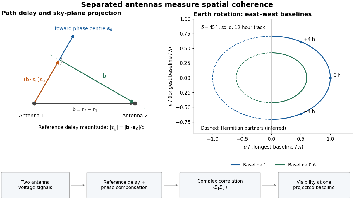
Geometric delay, projected baseline, and a schematic Earth-rotation track; original geometry, not telescope data
. Details. The left panel separates the component producing the reference delay from the component measuring angular structure. The right panel shows a possible Earth-rotation aperture synthesis track, with its opposite complex conjugate track. Those opposite samples provide the symmetry required by a real brightness distribution; they are not independent extra observations.
Earth-rotation aperture synthesis uses Earth's changing orientation to vary a fixed ground baseline's projection onto the plane of the sky. In two dimensions, and are the components of along two perpendicular sky tangents. Tracking one field traces a curve in this plane; changing the physical baseline supplies other curves. A track samples Fourier transform coordinates, rather than the brightness along a track across the sky.
For a horizontal east–west baseline of length , choose the sky-axis signs so thatwhere is hour angle and is declination. The ellipse follows by projecting the rotating baseline onto sky tangents. At a celestial pole it is a circle; near the celestial equator its minor axis collapses. Thus the same ground layout constrains different sky directions unequally. Rotation improves coverage, but does not fill every spatial frequency, and synthesis across many hours assumes that the source changes negligibly during that interval.
Radio interferometer calibration estimates instrumental and propagation effects that alter a complex visibility. A simple narrow-field model iswhere are complex receiver gains and represents additive noise. A point-like astronomical source of known position and stable strength constrains these gains: its expected complex visibility has a known wave phase and amplitude. A resolved or variable reference source requires a better source model. Errors in the reference model can be transferred into the inferred sky.
In a proposed extension, Martin Ryle described simultaneous observation of a nearby reference point source to correct atmospheric wave phase errors, using an additional dish at each element. He presented this as a possible extension, rather than the standard One-Mile Telescope arrangement.[ref]
Radio Telescopes of Large Resolving Power by Martin Ryle. Ryle (1974), p. 202: proposed reference-source correction
A complex visibility is a calibrated complex correlation of the signals received at a particular interferometric baseline. In a narrow field, with scalar radiation, the far-field approximation for an outgoing source, a narrow frequency channel, negligible noncoplanar phase curvature and a steady sky of mutually incoherent emitters,Here are small dimensionless sky-direction offsets, is brightness in the chosen channel, and is the primary beam. This is the Fourier transform of beam-weighted brightness. The two-dimensional formula requires those approximations: a wide field generally needs the third baseline coordinate and curved sky geometry.
For an explicit one-dimensional derivation, set the primary beam to one over the small field, and place independent emitters at angular offsets . Choose a wave phase convention in which, after removing the phase centre's delay, their received complex amplitudes areHere is the Kronecker delta and angle brackets denote an expected value estimated by time averaging a steady signal. The last equality states mutual incoherence: different emitters have zero averaged cross term, although each emitter's two received copies remain correlated. Multiplying and averaging givesFor continuous brightness this becomes . Real brightness implies the Hermitian symmetry ; it does not require brightness to be even. In particular, an asymmetric real source usually has a nonzero imaginary complex visibility. At zero baseline, is the total beam-weighted source strength. Ordinary separated-element correlations need not measure that zero-baseline value.
The primary beam is the individual antenna pair's directional sensitivity envelope in the complex visibility equation. For identical, identically pointed elements it is the individual element's power pattern. Its angular width sets the useful field of view; the much longer interferometric baselines set finer measured scales. The primary beam and the dirty beam describe different responses.
The One-Mile Telescope used three steerable 60-foot dishes: two fixed, one rail-mounted. The movable–fixed pairs supplied two baselines simultaneously. Twelve-hour tracks at successive rail positions sampled projected spacings. Phase-switching receivers measured in-phase and quadrature correlations; adjustable delay and phase rotation compensated tracking.[ref]
The Operation of the Cambridge One-Mile Diameter Radio Telescope by Bruce Elsmore and others. Elsmore et al. (1966), sections 1–2, pp. 87–92, Figures 1–2
The readout was correlation versus time. Reference-phase subtraction should leave constant point-source phase; position offsets produce predictable variation. A source near the field's declination supplies a collimation check. Structure, instrumental error and sampling artefacts need separating.[ref]
The Operation of the Cambridge One-Mile Diameter Radio Telescope by Bruce Elsmore and others. Elsmore et al. (1966), section 4(a), p. 93; Appendix, p. 95
The dirty beam is the point spread function obtained by directly inverting the weighted sampled complex visibilities. For sampling positions and nonnegative weights with , chooseInclude each with and the same weight so that is real. Its unit peak convention means that an isolated unit point source contributes a shifted unit-height response. It is not a unit-integral convention. Sparse sampling can leave substantial subsidiary peaks, even when the longest interferometric baseline is large.
The dirty image is the direct weighted inverse Fourier transform of the measured complex visibilities:The final equality follows by substituting the point-source complex visibility and exchanging the finite sums. For continuous brightness it is a convolution with the dirty beam, with the primary beam included in the brightness when necessary. Negative values and subsidiary peaks can arise from that response even when every true source has positive strength.
Choose two point-like astronomical sources with and , where the angles are in radians and strengths use arbitrary common units. Their separation is radians. These are invented model parameters, not historical measurements. Their complex visibility follows immediately from the preceding derivation, and its squared magnitude isAt , ; at , ; at , . The unequal strengths prevent the complex visibility magnitude from reaching zero. Its modulation contains the source separation, while a common displacement of both sources changes wave phase without changing this magnitude. Amplitude alone loses that location information.
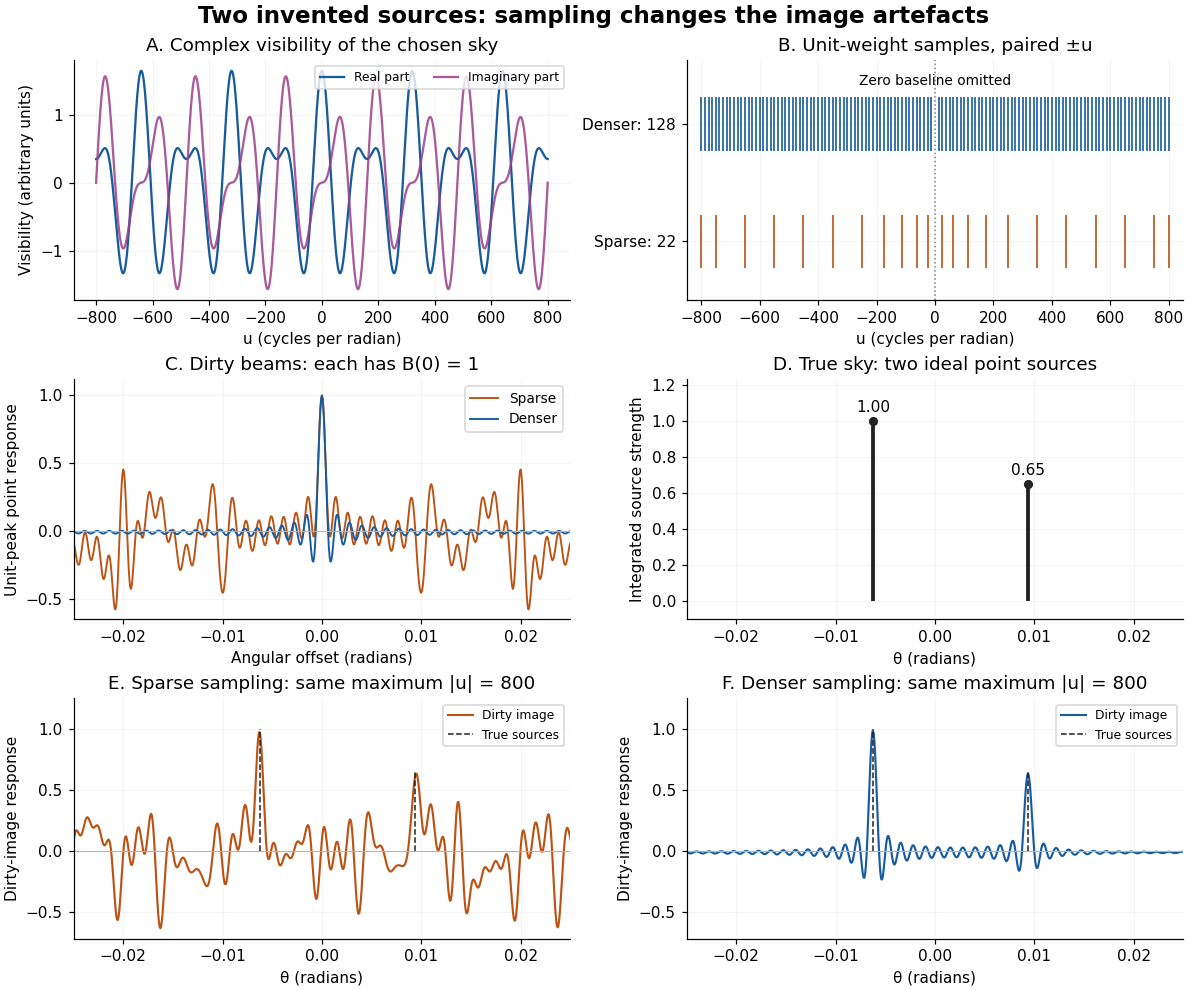
An original two-source model: complex visibility, sampling gaps, unit-peak dirty beams, and dirty images
. Details. The sparse case samples for ; the denser case samples every , also with both signs. All weights are one. Both reach , so their shortest fringe period is the same radians. Their dirty beams and false subsidiary features differ because the intermediate spatial frequencies differ. Neither case includes or frequencies above that maximum. The figure uses a periodic angular interval of length radians; this artificial boundary makes a discrete Fourier transform calculation exact for the chosen grid, rather than modelling an all-sky observation.
The plotted dirty image is the sum of two shifted dirty beams, not a fitted or deconvolved estimate of the source. Adding samples in this example reduces prominent spurious peaks; it does not establish a universal monotonic improvement for every weighting or sky. A missing zero baseline leaves the periodic dirty image with zero mean, so it cannot by itself recover the total positive brightness. Missing short spacings also weaken constraints on extended smooth emission.
Reconstruction is an inverse problem. A perturbation whose Fourier transform vanishes at every sampled coordinate can be added without changing the measurements: incomplete coverage leaves a null space. Nonnegative brightness, a restricted source region, or a model with a small number of components can reduce ambiguity, but each is additional information. Removing dirty beam artefacts means estimating a sky consistent with both data and such assumptions; a narrow central peak alone does not certify a unique image. Measurement error, uncertain calibration and source variability add further limitations.
Articles by others on the same topic



Radio astronomy is cool because it revealed:The 1974 Nobel Prize in Physics was awarded for pioneering radio astronomy from the late 40s onwards done at the University of Cambridge which was an epicenter of early research in that area, leading to the creation of the Mullard Radio Astronomy Observatory in 1958.
- some very interesting new types of astronomical objects that were not as noticeable in the visible spectrum notably:
- quasars: quasars are extremely redshifted, which means by Hubble's law that they are very far from Earth, so the fact that we could see them at all meant they must have produced immense amounts of light
- pulsars: scientists thought they had found extraterrestrial life when they saw these regularly pulsating signal sources!
- cosmic microwave background which is a major evidence for the Big Bang
- radio wavelengths penetrate Earth's atmosphere better than the visible spectrum making it easier to make ground-based observations