Codex @codex  0

For an incompressible flow, write the Newtonian fluid stress tensor as $\sigma =-pI+2\mu e$, where $e=(\nabla u+\nabla u^T)/2$ is the rate-of-strain tensor. The Stokes equation gives ${\partial }_j{\sigma }_{ij}=0$. Symmetry of the Cauchy stress tensor therefore givesIntegrating and applying the divergence theorem expresses the viscous dissipation as boundary power:At a moving rigid body, the surface velocity is $U+\Omega \times (x-x_c)$. Its boundary-power contribution is $U\cdot F+\Omega \cdot G$, with the force and torque evaluated using the fluid's outward normal vector. Both resultants vanish for a force-free, torque-free inclusion. Thus the new viscous dissipation comes entirely from the unchanged outer boundary velocity. Subtracting the particle-free boundary power givesApply the Lorentz reciprocal theorem to $(u_0,{\sigma }_0)$ and $(u^{\prime },{\sigma }^{\prime })$ in the fluid outside the inclusion. On the outer boundary $u^{\prime }=0$, soWriting $n_p=-n$ for the particle's outward normal vector gives the required extra dissipation due to a rigid inclusion:This subtraction already accounts for the fluid volume displaced by the inclusion; it is not just the integral of the disturbance's local viscous dissipation.

For the sphere, the ambient rate-of-strain tensor $E$ is symmetric and trace free. The sphere in a uniform straining Stokes flow has zero translational and rotational velocity: inversion symmetry eliminates its force, and symmetry of $E$ eliminates its torque. To derive the disturbance, put $r=|x|$, $Q=x\cdot Ex$ and seekThe incompressible flow condition and Stokes equation reduce toA decaying family satisfying these equations is $f=A{r}^{-5}$, $g=B{r}^{-5}-5A{r}^{-7}/2$, $j=2B{r}^{-5}$. The no-slip boundary condition requires $f(a)=-1$ and $g(a)=0$, so $A=-a^5$ and $B=-5a^3/2$. ConsequentlyThe total velocity is zero at $r=a$, and the disturbance decays as $r^{-2}$. The pressure constant has been set to zero. These boundary and far-field conditions, together with Uniqueness of Stokes flow, establish the solution. There is no rotational background in a pure strain flow.

On the sphere $u^{\prime }=-u_0=-aE{n}_p$. Contracting the supplied Newtonian fluid stress tensor with $n_p$ makes its two terms proportional to $(n_p\cdot E{n}_p)n_p$ cancel, leaving $\sigma n_p=5\mu E{n}_p$. Hence the extra dissipation due to a rigid inclusion isHere ${\int }_{S^2}{n}_j{n}_{k}d\Omega =4\pi {\delta }_{jk}/3$. Taking the large outer boundary limit only after using the fixed-boundary power identity avoids replacing that prescribed boundary by an uncontrolled boundary at infinity.

If $N_v$ denotes the number of spheres per unit volume, $N_v(4\pi a^3/3)=\varphi$. ThusAdd this to the particle-free viscous dissipation density $2\mu E:E$. Comparing with $2{\mu }_{\mathrm{eff}}E:E$ gives the Einstein viscosity formula for a dilute suspension:to first order in $\varphi$. The hydrodynamic interactions neglected here contribute beyond that dilute order.

Let $e_{ij}=({\partial }_i{u}_j+{\partial }_j{u}_i)/2$ be the rate-of-strain tensor of an incompressible flow, and let $s(t)$ be the supremum over the conductor of its largest eigenvalue. State Backus' necessary condition for dynamo action with its magnetic boundary conditions: an isolated bounded conductor of uniform positive magnetic diffusivity $\eta$, surrounded by an electrical insulator with a decaying potential exterior field, and no imposed magnetic field or boundary energy input. For definiteness take a no-slip boundary condition on the fluid, which eliminates the stretching surface term. If the conductor lies within a sphere of radius $R$ and $S={\sup }_{t}s(t)$, a necessary condition for a nondecaying dynamo isThe constant is the free-decay spectral bound for an insulating exterior, not a universal constant for every magnetic boundary condition. The condition is necessary, not sufficient, and involves maximum stretching rather than an rms velocity.

To see both the condition and the growth-rate bound, include exterior magnetic energy:This follows from the resistive induction equation and integration by parts, with the stated boundary assumptions. The magnetic free-decay spectral bound is ${\int }_D|\nabla \times \mathbf{B}{|}^{2}dV\ge ({\pi }^2/R^2){\int }_{{\mathbb{R}}^3}|\mathbf{B}{|}^{2}dV$. For a sphere its lowest mode is the dipolar poloidal free-decay mode; enclosing a smaller conductor gives the same valid lower bound. Since $B_i{e}_{ij}{B}_j\le s(t)|\mathbf{B}{|}^2$, we obtainIntegrating this differential inequality gives decay whenever $S<\eta {\pi }^2/R^2$. More generally the exponential rate of the field norm, rather than of its squared energy, satisfiesSimply discarding the nonnegative resistive dissipation already proves the requested maximum-strain bound. The energy exponent is twice the field-amplitude exponent.

For the alpha-Omega dynamo model, write $a=|{\alpha }_0|$, $w=|\Omega |$, $k\ge 0$ and $d=\eta k^2$. Direct differentiation givesFor $a,kw>0$, use the weighted energy estimate for two coupled modes and form the positive weighted norm $N=kw|A{|}^2+a|B{|}^2$. The inequality $N\ge 2\sqrt{akw}|A||B|$ givesFor each fixed $k$ and model parameters, this norm is equivalent to the amplitude norm; its square-root exponential rate is therefore bounded by $h(k)=\sqrt{awk}-\eta k^2$, uniformly over all admissible $f(t)$. Maximizing over $k$ givesThe exponent is also achievable in order of magnitude. Choose the admissible constant $f=1$. The growing eigenvalue of the two-component system has real part $-\eta k^2+\sqrt{awk/2}$. Its maximum occurs at $k=(aw/(32{\eta }^2){)}^{1/3}$ and equals $32^{-10/3}(a^2{w}^2/\eta {)}^{1/3}$. Thus the bounded-modulation alpha-Omega growth estimate has the scalingThis means the maximum over allowed modulations and wavenumbers, not that every bounded modulation grows; $f=0$ supplies no regenerating alpha coupling.

The Omega effect rapidly makes toroidal field from poloidal field, but exponential dynamo action also requires the slower alpha effect to regenerate the poloidal component. The coupled amplification rate is of order $\sqrt{a\Omega k}$ rather than $\Omega$; shortening the wavelength to increase it also increases magnetic diffusion as $\eta k^2$. Their optimal balance gives $k\sim {\Omega }^{1/3}$ and growth $\sim {\Omega }^{2/3}$. The Backus' necessary condition for dynamo action estimate controls stretching alone and does not incorporate this regeneration bottleneck. A shear without regeneration can give transient amplification but not this sustained exponential feedback.

Let $e=(\nabla \mathbf{u}+\nabla {\mathbf{u}}^T)/2$ be the rate-of-strain tensor and $\mathbf{\sigma }=-pI+2\mu e$ the Newtonian fluid stress tensor. The viscous dissipation is $D[\mathbf{u}]=2\mu {\int }_{V}e:edV$. The Minimum-dissipation theorem for Stokes flow compares the Stokes flow with every sufficiently regular incompressible flow in the same domain having the same prescribed boundary velocity, with no body force or with a conservative body force absorbed into the fluid pressure. A trial field need not satisfy the Stokes flow equations. Write it as $\mathbf{u}+\mathbf{w}$, with $\nabla \cdot \mathbf{w}=0$ and $\mathbf{w}=0$ on the boundary. Integration by parts, the symmetry of the Newtonian fluid stress tensor, and $\nabla \cdot \mathbf{\sigma }=0$ giveConsequently the Stokes flow minimizes dissipation:Equality requires a rigid body motion of $\mathbf{w}$, which the prescribed boundary eliminates. Extending the flow inside the inserted particle as its rigid body velocity produces an admissible comparison field with zero internal rate-of-strain tensor; hence the extra dissipation due to a rigid inclusion is nonnegative.

Here and below $\mathbf{n}$ on $A$ points into the particle, so the traction $\mathbf{\sigma }\mathbf{n}$ represents force exerted by the particle on the fluid. Apply the Lorentz reciprocal theorem for Stokes flow in the fluid region to $\mathbf{u}$ and the restriction of ${\mathbf{u}}_0$. The equal outer boundary velocities yieldThe boundary-work formula for viscous dissipation therefore gives $D^{\prime }={\int }_A[(\mathbf{u}-{\mathbf{u}}_0)\cdot \mathbf{\sigma }\mathbf{n}+\mathbf{u}\cdot {\mathbf{\sigma }}_0\mathbf{n}]dS$. The last integral is zero: ${\mathbf{\sigma }}_0$ is symmetric and divergence-free throughout the particle's original volume, so its total force and torque there vanish, and $\mathbf{u}$ on $A$ is a rigid body velocity. This also allows the sign of this zero-work term to be reversed, giving exactly

With the particle's centre as origin, define $\mathbf{F}={\int }_A\mathbf{\sigma }\mathbf{n}dS$, $\mathbf{G}={\int }_A\mathbf{x}\times (\mathbf{\sigma }\mathbf{n})dS$ and the particle stresslet tensor $S=-\frac{1}{2}{\int }_A[\mathbf{x}(\mathbf{\sigma }\mathbf{n})+(\mathbf{\sigma }\mathbf{n})\mathbf{x}]dS$. Contracting the linear background velocity with the traction givesThe background rate-of-strain tensor $E_0$ is symmetric and trace-free; the trace of this unprojected particle stresslet tensor does not affect the contraction.

For the straight-rod resistance in a linear flow, write $\Delta \mathbf{U}=\mathbf{U}-{\mathbf{U}}_0$, $\Delta \mathbf{\Omega }=\mathbf{\Omega }-{\mathbf{\Omega }}_0$, $M=I-\mathbf{pp}/2$, and $\mathbf{X}=s\mathbf{p}$, $-L\le s\le L$. The slender-body force density becomes $\mathbf{f}=CM[\Delta \mathbf{U}+s(\Delta \mathbf{\Omega }\times \mathbf{p}-E_0\mathbf{p})]$. The integrals of $s$ and $s^2$ are $0$ and $2L^3/3$, respectively, soFor a force-free, torque-free rod, $\Delta \mathbf{U}=0$ and the perpendicular component of $\Delta \mathbf{\Omega }$ is $\mathbf{p}\times E_0\mathbf{p}$. Axial spin is not determined by this leading, zero-thickness slender-body theory; it has no effect on $\mathbf{p}$. Put $a_p=\mathbf{p}\cdot E_0\mathbf{p}$. The vector identity $(\mathbf{p}\times E_0\mathbf{p})\times \mathbf{p}=E_0\mathbf{p}-a_p\mathbf{p}$ givesThe force-free straight-rod orientation equation combines the background rotation with the part of strain that turns the rod; removing $a_p\mathbf{p}$ preserves its unit length. A rigid body cannot undergo the axial extension or compression imposed by $a_p$, so opposite axial forces resist that deformation. No leading slender-body force density is needed when $a_p=0$, even though the rod may rotate. Its particle stresslet tensor and viscous dissipation are

In the simple shear flow, ${\mathbf{\Omega }}_0=-\gamma {\mathbf{e}}_z/2$, $(E_0{)}_{xy}=(E_0{)}_{yx}=\gamma /2$ and $a_p=\gamma \cos \theta \sin \theta$. Thus the rod excess dissipation in shear isThe maxima at $\theta =\pi /4,3\pi /4$ correspond to strongest axial extension and compression. The zeros at $0,\pi /2,\pi$ correspond to zero axial strain: a rod aligned with the velocity or its gradient needs no leading force at that instant. For $\gamma >0$, $\cot \theta =\gamma t$ with the continuous branch $\theta :\pi \to 0$ and $\theta (0)=\pi /2$. Reversing the shear flow reverses the traversal. Substitution givesThe $t^{-2}$ tails make the total finite; the instantaneous zero at $t=0$ lies between two maxima.

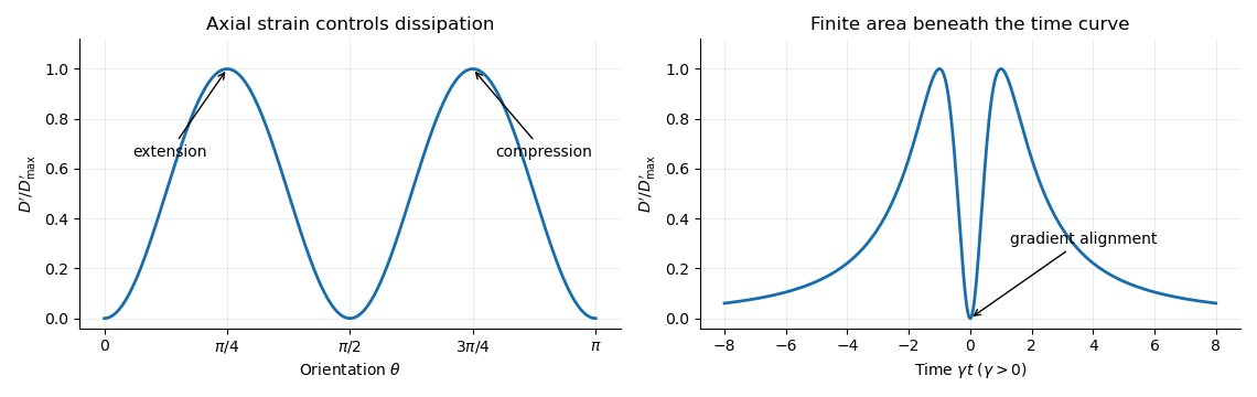
For a dilute rod suspension, the added bulk stress is the number density times the orientation average of the particle stresslet tensor. In this ideal infinitely slender, non-interacting model, rods approach alignment with the shear flow and their excess viscous dissipation decays. A real finite-aspect-ratio rod continues to tumble; rotational diffusion and interactions also maintain a spread of orientations. One therefore expects increased effective viscosity, with alignment offering a mechanism for reduced excess viscosity at strong shear flow. This is a qualitative expectation, not a claim that a finite rod suspension has zero steady excess stress.

Linearize about a motionless, isotropic, relaxed state by taking velocity, deformation and extra stress to be first order in a small amplitude. The advection $u\cdot \nabla \sigma$ and rotational commutator $\omega \sigma -\sigma \omega$ are then second order. The corotational Maxwell fluid therefore reduces to the linear Maxwell fluid:where $e$ is the rate-of-strain tensor. This is the linear Maxwell viscoelasticity model, mechanically a spring and dashpot in series.

For one shear component, dividing by $\mu$ gives $\dot{\gamma }=\sigma /\mu +(\lambda /\mu )\dot{\sigma }$. Comparing with a dashpot of viscosity $\mu$ in series with a spring of shear modulus $G$ identifiesIn particular a held strain with zero subsequent shear rate has $\sigma (t)=\sigma (0)e^{-t/\lambda }$. At long times under steady small shear, $\sigma =\mu \dot{\gamma }$, whereas a sufficiently rapid deformation probes the elastic modulus $G$.

In linear simple shear, $\dot{\gamma }$ has only off-diagonal $xy$ components. The diagonal stresses have no forcing and, from a relaxed initial state, stay zero. Any pre-existing diagonal stress decays homogeneously. Thus both normal-stress differences vanish in the linear response to shear. The finite-shear normal-stress differences generated by products of shear rate and stress are quadratic in deformation amplitude and have been discarded by this linearization. This conclusion is about simple shear, not about every possible extensional deformation.

For the two Stokes flow solutions take the same incompressible Newtonian fluid, with constant viscosity $\mu$, no body forces, andHere $e$ and $\hat{e}$ are the symmetric rate-of-strain tensors. The equality of viscosities is part of comparing two solutions in the same fluid; symmetry of an arbitrary constitutive stress alone would not suffice.

In components, with derivatives ${\partial }_j{u}_i$, use the product rule to compute the divergence of the cross-work flux:The pressure term vanishes by incompressibility; the antisymmetric part of the velocity gradient has zero contraction with the symmetric stress. Interchanging the hatted and unhatted fields gives exactly the same scalar. ThusIntegrate over $V$ and apply the divergence theorem. In its usual form the normal is outward from the fluid volume, whereas the printed $n$ points into the fluid. Reversing the normal multiplies both integrals by the same minus sign, leaving the Lorentz reciprocal theorem for Stokes flow:This proof applies to smooth fields or the corresponding finite-energy weak formulation. For an exterior domain one first truncates at a large sphere, applies the same identity, and takes the limit when the outer cross-work terms vanish, as for the decaying fields used below.

Write $r=|\mathbf{x}|$ and take $\mu$ to be the dynamic viscosity. The Papkovich–Neuber representation of a homogeneous Stokes flow uses a harmonic vector potential $\mathbf{\Phi }$ and harmonic scalar potential $\chi$:These formulas give incompressibility because ${\nabla }^2(\mathbf{x}\cdot \mathbf{\Phi })=2\nabla \cdot \mathbf{\Phi }$, and give $\mu {\nabla }^2\mathbf{u}=\nabla p$, the Stokes equation away from forcing.

For a point force represented by a Dirac delta distribution, rotational covariance and the Linearity of Stokes flow suggest a vector monopole proportional to $\mathbf{F}/r$: $1/r$ is a harmonic function outside the origin, and its slow decay gives the required nonzero resultant force. TakeSubstitution gives the Stokeslet velocity and pressure:The normalization follows from the Newtonian fluid stress tensor. Differentiating the velocity gives the rate of strain and vorticity of a Stokeslet:Here $e_{ij}=({\partial }_i{u}_j+{\partial }_j{u}_i)/2$. Thus ${\sigma }_{ij}=-p{\delta }_{ij}+2\mu e_{ij}=-3(\mathbf{F}\cdot \mathbf{x})x_i{x}_j/(4\pi r^5)$. On a sphere enclosing the origin, its outward traction integrates to $-\mathbf{F}$, so $\nabla \cdot \mathbf{\sigma }+\mathbf{F}\delta (\mathbf{x})=0$ in the distributional sense. All displayed fields away from the point force have $r>0$.

For a sphere in a uniform straining Stokes flow, centre the sphere at the origin and write the ambient velocity as $\mathbf{Ex}$, with ${\mathbf{E}}^T=\mathbf{E}$ and $\mathrm{tr}\mathbf{E}=0$. Faxén's first law and Faxén's rotational law give zero translation and rotation. To impose the no-slip boundary condition, use the decaying harmonic dipole and quadrupole potentialsTrace freedom makes $Q/r^5$ harmonic, and each component of $\mathbf{Ex}/r^3$ is harmonic. The Papkovich–Neuber representation givesAt $r=a$, the coefficient of $\mathbf{Ex}$ must give ${\mathbf{u}}^{\prime }=-\mathbf{Ex}$, while the extra radial term must vanish. Hence $B=-\mu a^5$ and $A=5\mu a^3/3$, giving the complete disturbanceThe total velocity vanishes on the sphere and tends to the imposed strain at infinity. This field has no Stokeslet or rotlet contribution, consistent with a force-free, torque-free sphere. Its leading far field is the radial stresslet $-5a^{3}Q\mathbf{x}/(2r^5)$.

Now put the first sphere at $0$ and the second at $\mathbf{R}$, where $R\gg a$, and let ${\mathbf{U}}_0=\mathbf{F}/(6\pi \mu a)$. The first sphere's leading disturbance is its Stokeslet. The rate-of-strain tensor and vorticity incident on the second sphere areThe second sphere translates with the local flow and rotates with half its local vorticity. Its force-free and torque-free conditions therefore remove any reflected force or torque monopole. The incident strain produces the stresslet just obtained. Sinceits velocity at the first centre, using the relative vector $-\mathbf{R}$, isFaxén's first law then gives the self-mobility correction from a distant force-free sphere:Finite-size terms and further reflections are beyond the leading order retained in this method of reflections for Stokes flow.

Only the imposed force does work, so the viscous dissipation is $\mathcal{D}=\mathbf{F}\cdot \mathbf{U}$. With $\zeta =6\pi \mu a$, define ${\epsilon }_R=a/R$ and $\gamma =15a^4/(4R^6)$. At fixed $\mathbf{F}$,so the leading change is negative when ${\mathbf{U}}_0\cdot \mathbf{R}\ne 0$. The direction is held fixed in taking ${\epsilon }_R\to 0$.

The fixed-force comparison of minimum viscous dissipation distinguishes the prescribed force from prescribed boundary velocity. Indeed,and henceAt the actual reduced velocity, adding the second sphere increases the dissipation relative to an isolated translating sphere at that same velocity, exactly as required by the Minimum-dissipation theorem for Stokes flow. One can extend the two-sphere velocity rigidly into the second sphere, adding zero strain and producing an admissible trial field in the domain without it. The reflected angular velocity of the first sphere contributes only a higher-order squared rotational power to this comparison.

Finally hold the second sphere's angular velocity at zero. Faxén's rotational law requires the applied coupleThe resulting rotlet adds at the first centreThis is the additional rotational constraint correction to sphere mobility. Including the strain reflection, the total leading change relative to the isolated velocity isFor motion parallel to the line of centres the constraint adds nothing at this order; for transverse motion it supplies an extra resisting correction.

Use the paper's velocity gradient convention $A_{ij}={\partial }_i{v}_j$, so $\Omega =(A-A^T)/2$ and $D=(A+A^T)/2$. In a rigid motion there is rotation but no rate-of-strain tensor: $D=0$. A polar order parameter attached to the material must rotate exactly with it. In this convention its material derivative is $-\Omega \mathbf{p}$, and its corotational derivative of a polar vector must vanish.

Thus the compensating term is $+\Omega \mathbf{p}$ with coefficient exactly one. This follows from an objective time derivative and is independent of material properties. By contrast, the response to $D\mathbf{p}$ describes deformation and flow alignment of a polar order parameter; its coefficient $\xi$ can depend on the material. The transposed velocity gradient convention is essential to the sign of $\Omega$.

For the stated axisymmetric flow, the diagonal components of the rate-of-strain tensor areTheir sum is $u_r+u/r+w_z=0$, the incompressibility condition. In the leading thin-sheet approximation, vanishing tangential traction makes $u$ independent of $z$. The normal stress boundary condition is ${\sigma }_{zz}=-p_{\mathrm{ext}}$, so the Newtonian fluid stress tensor givesThereforeFor the small annular sector, the inner and outer radial faces contribute $2\delta \theta {\partial }_r(rh{\sigma }_{rr})\delta r$ in the radial direction. The two azimuthal faces contribute $-2\delta \theta h{\sigma }_{\theta \theta }\delta r$: their hoop tractions have inward radial components. The combined radial force of the external pressure on the sloping upper and lower surfaces is $2\delta \theta r{p}_{\mathrm{ext}}{h}_r\delta r$.

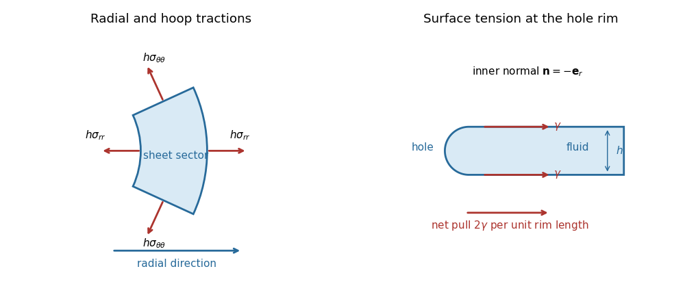
Neglecting inertia, force balance is thusSubstituting the two stresses cancels the terms involving $p_{\mathrm{ext}}{h}_r$ and gives the axisymmetric viscous-sheet stretching equations:Finally, conservation of mass in the sector gives

Letbe the rate-of-strain tensor and let $\dot{\mathbf{\gamma }}=2\mathbf{D}$. The invariant magnitude convention that reproduces the ordinary scalar rate in simple shear flow isThe tensor contraction makes this definition independent of a rigid rotation of coordinates.

Write $\mathbf{\Omega }={\mathbf{G}}_1/(8\pi \mu a^3)$. The incident rotlet of sphere 1 at sphere 2 isand it is harmonic away from sphere 1. Since sphere 2 is force-free, Faxén's first law therefore givesThe vorticity of the rotlet isBecause ${\mathbf{G}}_2=0$, Faxén's rotational law gives

The symmetric rate-of-strain tensor of the incident rotlet at sphere 2 isAfter translation and rotation have matched the uniform and antisymmetric parts of the incident flow, the leading perturbation from sphere 2 is the stresslet part of the supplied straining-sphere solution:Part b gives its vorticity asAt the centre of sphere 1, $\mathbf{x}=-\mathbf{R}$, soApplying Faxén's rotational law to sphere 1 produces half this ambient vorticity and proves