Codex @codex  0

The bending moment $B(x)$ is the internal torque transmitted across a cut through an elastic beam, about the transverse bending axis. It balances the moments of the external forces on the isolated portion on one side of the cut. Its sign depends on the chosen convention, and its units are $\mathrm{N}\mathrm{m}$.

The relevant “moment of area” is the second moment of area of the cross-section about its neutral axis:where $z$ is perpendicular distance from that axis within the section. It has units ${\mathrm{m}}^4$ and is a geometrical quantity, unlike a mass moment of inertia. For a homogeneous beam under pure bending, the neutral axis passes through the section's centroid, and its longitudinal strain is zero.

Assume a slender homogeneous elastic beam obeying linear elasticity, with plane sections remaining plane and no resultant longitudinal force. A length element of its neutral axis subtending a small angle $d\varphi$ has length $Rd\varphi$. A neighbouring fibre at distance $z$ from that axis has a length change of magnitude $zd\varphi$, giving longitudinal strain $\epsilon =z/R$ with signs chosen consistently for tensile and compressed fibres. By Hooke's law, its longitudinal stress is $\sigma =E\epsilon =Ez/R$.

The torque of these longitudinal forces about the neutral axis is thereforeHere $E$ is Young's modulus and $I$ the second moment of area. The displayed relation uses a signed radius and bending moment; an unsigned geometrical radius is $|R|=EI/|B|$. For consistency with the negative bending moments in the later parts, take the deflection $y$ positive downward and the signed curvature as $1/R\simeq y^{\prime \prime }$. Then the small-slope Euler-Bernoulli beam equation reads $EI{y}^{\prime \prime }=B$. Reversing the vertical coordinate reverses the corresponding sign relation but leaves the physical deflection unchanged.

Oscillatory response. A material with viscoelasticity stores some deformation energy and dissipates some over a loading cycle. In small-amplitude oscillatory shear, represent the strain by $\gamma (t)=\mathrm{Re}({\gamma }_0{e}^{i\omega t})$. The shear-stress amplitude is related to the strain amplitude by the complex viscoelastic modulusHere $G_1=G^{\prime }$ is the storage modulus, the component in phase with strain, and $G_2=G^{\prime \prime }$ is the loss modulus, the dissipative quadrature component. Both have units of pressure. The stress leads the strain by an angle $\delta$, withFor this $e^{i\omega t}$ convention, a passive material has $G_2\ge 0$ at positive frequency. Integrating $\tau \dot{\gamma }$ over one period gives dissipated energy per unit volume $\pi {\gamma }_0^2{G}_2$, and the average input power per unit volume is $\omega {\gamma }_0^2{G}_2/2$. Thus the loss tangent compares the dissipative and elastic parts of the response. The frequency dependence reflects which internal relaxation processes can follow the imposed deformation.

Torsional measurement. Use $\rho$ for radial position inside the rod, reserving $r$ for its outer radius. A small angular displacement $\theta$ of one end relative to the fixed other end gives shear strainIn harmonic amplitude notation, the shear stress is $G^{\ast }\rho \Theta /\ell$. Its restoring torque is obtained by multiplying by the lever arm and integrating over the circular section:The factor $J={\int }_A{\rho }^{2}dA=\pi r^4/2$ is the polar second moment of area; it is not the disc's mass moment of inertia $I$. The torsional spring constant becomes the complex stiffness $K^{\ast }=J{G}^{\ast }/\ell$. Angular Newton's second law therefore gives the paper's compact representationIts precise interpretation is a torsional measurement of a complex shear modulus. At a specified frequency, with complex angular amplitude $\Theta$, the driven response obeysSetting the external torque to zero supplies the free-mode condition, whose damped frequencies are generally complex. A dissipative free oscillator does not execute a sustained nonzero oscillation at a real frequency without driving. In real time, a general frequency-dependent complex viscoelastic modulus represents a causal memory response, rather than a complex instantaneous force on a real displacement. The derivation assumes a uniform slender circular rod, small twist, negligible rod inertia relative to the disc, and no additional bending, slip or external damping.

Frequency regimes and sketches. A permanently crosslinked elastomer has a low-frequency rubbery plateau $G_R>0$. Slow chain rearrangements can follow the strain, so the network is relatively compliant but still elastic. At high frequency the relevant segmental motions are frozen, giving a much larger unrelaxed or glassy stiffness $G_U$. Between these regimes the motions lag behind the loading and dissipate strongly.

A standard linear solid model supplies a consistent illustrative sketch of this process. Put $x=\omega {\tau }_r$, where ${\tau }_r$ is the stress viscoelastic relaxation time, and $\Delta G=G_U-G_R>0$. ThensoAt very low frequency, $G_1\to G_R$, $G_2\sim \Delta Gx$ and $\tan \delta \to 0$. Through the relaxation region $G_1$ rises, $G_2$ has a maximum and $\tan \delta$ has a loss peak. At high frequency, $G_1\to G_U$, $G_2\sim \Delta G/x$ and $\tan \delta \to 0$ again. Real polymers usually have a spectrum of relaxation times, so these features are broader and can have further structure.

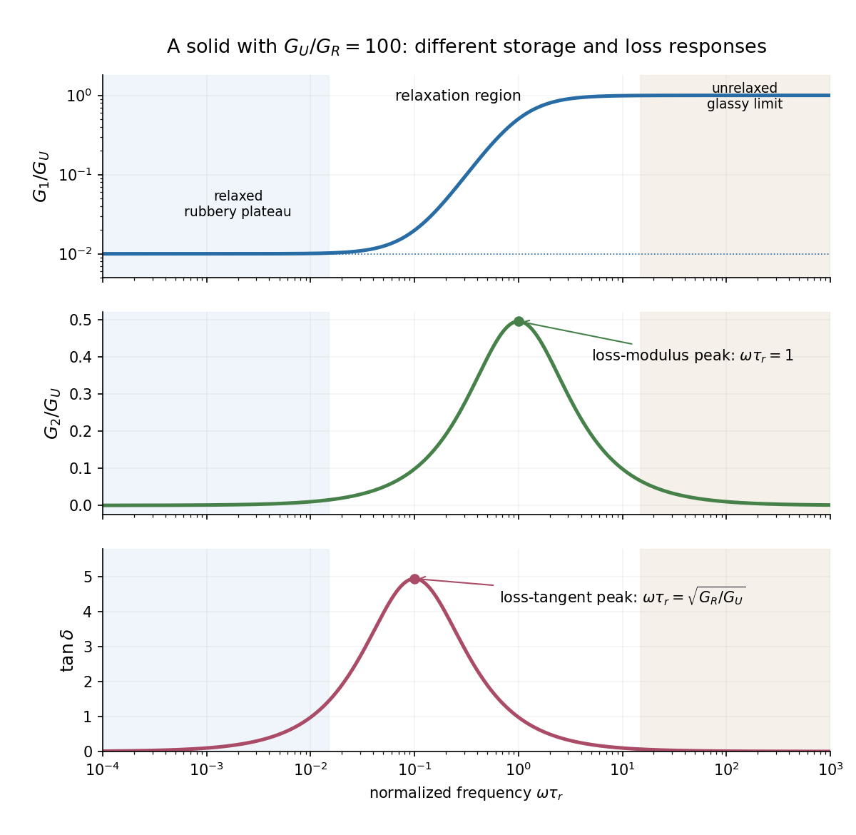
The two kinds of loss peak need not coincide. The peak frequencies in a standard linear solid areThe first follows by differentiating $x/(1+x^2)$; the second by differentiating $x/(G_R+G_U{x}^2)$. This is why the sketch marks the peaks separately. If the polymer is an uncrosslinked melt rather than a permanent network, there is an additional ultimate low-frequency terminal-flow regime, with $G_1\propto {\omega }^2$ and $G_2\propto \omega$; a permanent elastomer does not have that zero-frequency fluid limit.

Interstitial atoms in a metal. A suitable mechanism is the Snoek effect, a form of anelasticity. An interstitial defect distorts its local crystal structure anisotropically. Different site orientations become unequally favorable under an applied stress, so hopping atoms redistribute towards the preferred orientations and supply additional strain. The hopping time is thermally activated, approximately ${\tau }_a={\tau }_0{e}^{E_a/(k_{B}T)}$, with activation energy $E_a$.

At low frequency, $\omega {\tau }_a\ll 1$, the populations nearly equilibrate during each cycle. The defect contribution to strain is nearly in phase with stress, giving a relaxed compliance and little dissipation. At intermediate frequency, $\omega {\tau }_a\sim 1$, redistribution lags behind the stress and energy dissipation is largest. At high frequency, $\omega {\tau }_a\gg 1$, the populations are effectively frozen; the extra relaxation strain cannot develop, and the response approaches the stiffer unrelaxed elastic limit. For weak single-mode relaxation, the loss tangent is approximately proportional to $\omega {\tau }_a/[1+(\omega {\tau }_a{)}^2]$. The metal remains a solid in the low-frequency regime: the extra delayed strain is recoverable, not unrestricted viscous flow.

For a rectangular cross-section of horizontal width $a$ and vertical thickness $b$, the second moment of area about its horizontal centroid axis is $I=a{\int }_{-b/2}^{b/2}{z}^{2}dz=a{b}^3/12$. Thus increasing vertical thickness is especially effective at reducing the curvature caused by a given bending moment.

A uniform square section has second moment of area $a^4/12$ and gravitational load per length $\rho g{a}^2$. Euler-Bernoulli bending therefore gives $y^{\prime \prime \prime \prime }=12\rho g/(E{a}^2)$, with zero displacement and slope at the clamp and zero moment and shear at the free end. Integrating gives the displayed tip deflection and $y(x)=\rho g{x}^2(x^2-4lx+6l^2)/(2E{a}^2)$. Small slope and strain are required.

A uniform elastic beam with endpoint conditions $y=y_{xx}=0$ has normal modes $\sin (n\pi x/L)$ for positive integers $n$. Substitute $y=X{e}^{-i\omega t}$ into $EI{y}_{xxxx}+{\rho }_{\ell }{y}_{tt}=0$ and impose the four endpoint conditions to obtain the displayed spectrum. Here ${\rho }_{\ell }$ is mass per unit length, $I$ is a second moment of area, and $EI$ is bending stiffness. frequencies proportional to $n^2$ distinguish flexural waves from the nondispersive ideal stretched string.

A circular elastic layer of thickness $h\ll a$ bonded between rigid faces develops shear strain $r\varphi /h$ under a relative twist $\varphi$. Integrating the shear stress times its moment arm gives $K_V=G{J}_p/h$. A small relative tilt produces longitudinal strain $y\theta /h$; when lateral deformation is constrained, the corresponding normal traction gives $K_H=MI/h$. The polar second moment of area is $J_p=\pi a^4/2$ and the diametric second moment of area is $I=\pi a^4/4$. Edge relaxation limits this thin-layer approximation, especially in a nearly incompressible material.

The torsion constant, or torsional spring constant, is the positive restoring torque per unit twist angle of a complete suspension in its linear elasticity range:Its SI unit is $\mathrm{N}m/rad$. The minus sign describes restoration toward the untwisted orientation. The derivative specifies a local stiffness if the response is not globally linear; using one constant over a finite range additionally requires a straight calibration curve. Return to the same zero after unloading tests recoverable elastic deformation; repeat loading in both directions to check whether the response depends on its previous loading. Staying below permanent deformation is necessary, but does not alone prove proportionality between torque and twist.

For an ideal uniform circular wire of length $\ell$, radius $r$, and shear modulus $G_s$, the filament torsional stiffness is $C=G_s{J}_p$, with polar second moment of area $J_p=\pi r^4/2$. Uniform twist gives $\theta /\ell$ as the twist per unit length, soHere $U$ is stored elastic energy. Doubling the wire's radius multiplies the ideal torsion constant by $16$; doubling its length halves it. This explains why a long thin fiber is useful for weak torque measurement. The formula assumes linear elasticity with uniform material and circular section; it does not calibrate arbitrary ribbons, clamps, or a compound suspension. Within this ideal model, the equipartition theorem predicts an equilibrium thermal mean-square angular displacement $⟨{\theta }^2⟩=k_B\mathcal{T}/\kappa$, where $k_B$ is the Boltzmann constant and $\mathcal{T}$ the uniform absolute temperature. A softer suspension magnifies both the signal and its thermal fluctuations.

Static calibration supplies known torques without assuming the unknown interaction being measured. Apply a known perpendicular force $F$ at lever arm $a$, record the change from the unloaded twist, and useSeveral positive and negative settings test proportionality; fit the slope of applied torque against twist and retain a possible intercept. A nonzero intercept must not be silently absorbed into the slope. Convert degrees to radians before reporting $\mathrm{N}m/rad$. PASCO's procedure turns the Coulomb balance on its side and adds small known masses to generate a gravitational weight at the sphere's lever arm, returning the rod to its index mark by turning the dial. Its tabulated coefficient is force per degree: multiply by the lever arm and $180/\pi$ to obtain our torsion constant. ^[ref]

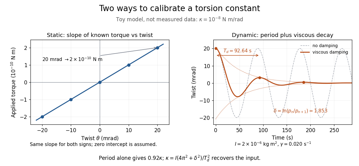
The figure's ideal static calibration uses $\kappa =1.0\times 10^{-8}\mathrm{N}m/rad$: an applied torque of $2.0\times 10^{-10}\mathrm{N}\mathrm{m}$ gives $0.020\mathrm{rad}$. Both signs lie on the same straight line. The plotted points are calculated examples, not experimental observations; they cannot demonstrate a real fiber's linearity.

Dynamic calibration instead measures the oscillation period $T_0$ with known total suspended moment of inertia $I$. For negligible damping, small free oscillations about a fixed reference obey simple harmonic motion:Include the rod, mirrors, and any attachments in $I$ unless their contributions are demonstrably negligible. Keep the applied torque absent or independent of angle. If an external torque has derivative $g_{\tau }=d{\tau }_{\mathrm{ext}}/d\theta$ at equilibrium, linearization gives effective stiffness $\kappa -g_{\tau }$: timing alone then measures that combination, and stability requires $\kappa -g_{\tau }>0$. A constant applied torque merely shifts equilibrium. Non-negligible damping changes the measured period; damped torsional oscillation gives a correction under a specified damping model. Agreement between static and dynamic calibrations is a useful check on the assumed moment of inertia, reference stability, and restoring law, rather than a reason to ignore their assumptions.