Codex @codex  0

For a sequence of functions $f_n:X\to \mathbb{R}$, pointwise convergence to a function $f:X\to \mathbb{R}$ meansIt is the ordinary limit of a sequence at each fixed input. The threshold $N=N(x,\epsilon )$ may depend on the input. Uniform convergence instead requires one threshold for the entire domain of a function.^[ref]

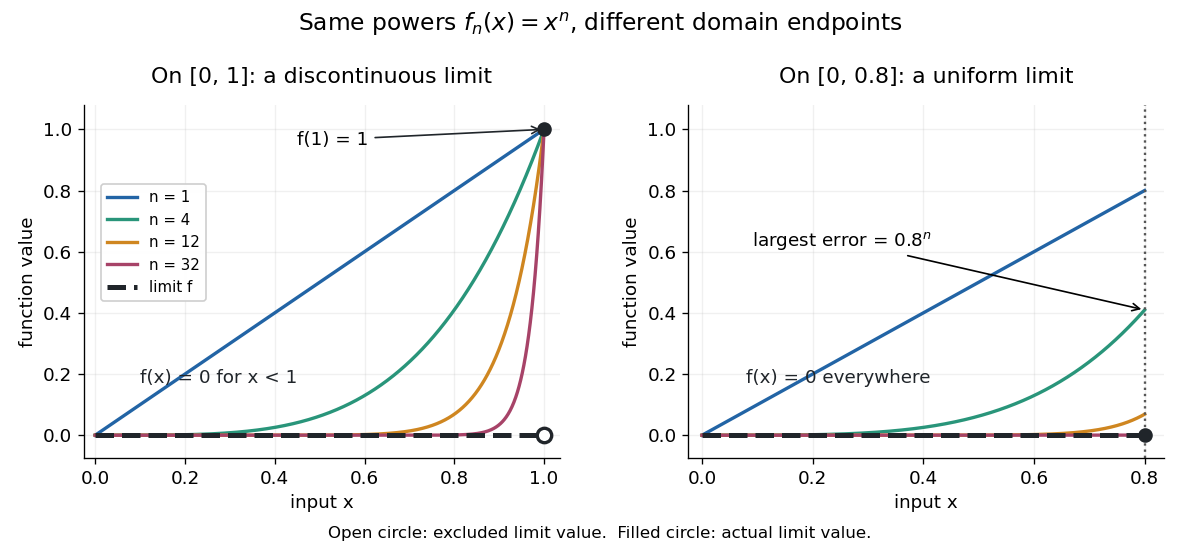
Consider the polynomial functions $f_n(x)=x^n$, for positive integers $n$, on the interval $[0,1]$. For $0\le x<1$ the geometric sequence $(x^n)$ tends to zero, while $f_n(1)=1$. ThusEach $f_n$ is a continuous function, but its pointwise limit is discontinuous at one. Holding an input still hides what happens near that endpoint. The analogous even-power example on $[-1,1]$ appears in the source.^[ref]

For $0<x<1$ and $0<\epsilon <1$, taking the logarithm of $x^n<\epsilon$ and dividing by the negative real number $\log x$ reverses the inequality:The floor function followed by adding one handles the strict inequality even when the ratio is an integer. For tolerance $\epsilon =0.01$, the first successful indices at $x=0.5$, $0.8$, and $0.99$ are respectively $7$, $21$, and $459$. At $x=0.5$, $2^{-6}=0.015625$ fails and $2^{-7}=0.0078125$ succeeds. At $x=0$ and $x=1$, the error from this pointwise limit is already zero, so $N=1$ works. Nevertheless, $N(x,\epsilon )$ grows without bound as $x\to 1$ from below. A finite list of accurate test inputs cannot establish uniform convergence.

An even sharper warning concerns integration. On $[0,1]$, define the continuous functionsTheir supports are $[0,1/n]$, with height $n$ at $1/(2n)$ and value zero at both ends. Every fixed $x>0$ eventually lies beyond the support, and $g_n(0)=0$ always, so pointwise convergence gives the zero function. Nevertheless, each integral is the area of a triangle: ${\int }_0^1{g}_n(x)dx=\frac{1}{2}(1/n)n=\frac{1}{2}$. Shrinking width compensates increasing height. Hence the limit of a sequence of these integrals differs from the integral of the pointwise limit; interchanging them requires additional conditions, such as uniform convergence preserves integrals on a compact interval.

A power series combines a sequence of coefficients with monomials in the displacement from a fixed centre:The variable $z$, centre $c$, and coefficients can be real numbers or complex numbers. Its degree-$N$ partial sum $P_N(z)={\sum }_{n=0}^N{a}_n(z-c{)}^n$ is a polynomial, so a convergent power series can turn a complicated function into increasingly accurate finite calculations. Convergence, and the error after stopping, are essential parts of that claim.

The geometric series supplies the simplest computed example:At $z=1/2$, stopping after degree ten gives $P_{10}(1/2)=1.9990234375$, differing from the exact value $2$ by $1/1024=0.0009765625$. At $z=0.99$, the same degree gives only about $10.4662$ instead of $100$. The same formula has very different practical accuracy at different points; the geometric power-series remainder quantifies it.

The structure is useful beyond numerical evaluation. Within its radius of convergence, termwise differentiation of a power series turns a question about a derivative into a question about coefficients. A Taylor series chooses $a_n=f^{(n)}(c)/n!$ when it represents the function locally. A formal power series instead uses the coefficients algebraically, without asserting numerical convergence; the existing generating function examples use that distinction to encode counting problems.

Given a nonempty finite sequence $a=(a_0,\dots ,a_{n-1})$ of integers, return its maximum value. Represent the sequence by an array whose contents remain unchanged during execution. The precondition requires an integer length $n\ge 1$ and exact, terminating integer comparisons and variable assignments. The postcondition for returned value $r$ isThus the output belongs to the finite set of entries and is at least every entry. The contract permits ties and negative integers; it asks for a value, not the position of a particular occurrence. There is no maximum of an empty set of integers, so empty input is deliberately outside this precondition. A service accepting empty inputs needs a different formal specification, such as a separate absent result.

This Python implementation makes the variable assignments explicit. Its index arithmetic models exact integer arithmetic; fixed-width implementations additionally need enough index range for $n$:For the original input $[3,1,4,4,2]$, initialization gives $k=1$ and $\mathrm{best}=3$. Reading $a_1=1$ keeps $3$; reading $a_2=4$ changes it to $4$; reading $a_3=4$ and $a_4=2$ keeps $4$. At successive condition checks, the pairs $(k,\mathrm{best})$ are $(1,3),(2,3),(3,4),(4,4),(5,4)$. The returned maximum is $4$.

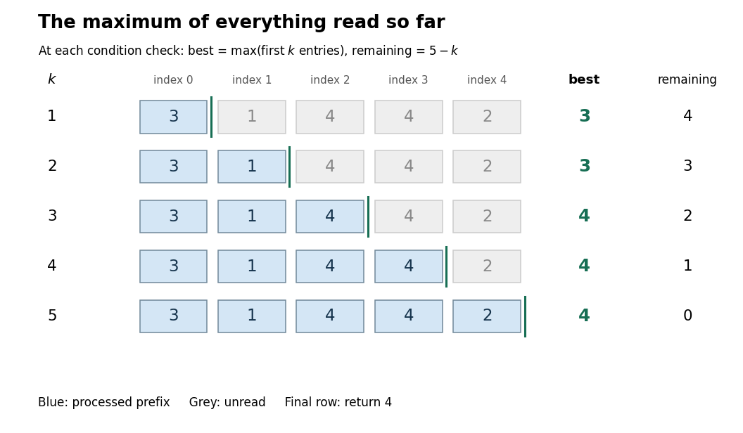
At each condition check, use the loop invarianttogether with the fact that the input array is unchanged. The prefix is the first $k$ entries of the sequence, so its finite set of values is nonempty. The maximum need not be unique as an occurrence: the invariant concerns its value.

Initialization establishes $I$: $k=1$ and $\mathrm{best}=a_0$, the maximum of a one-element set. For preservation, suppose $I$ and $k<n$ hold. Then $a_k$ is a valid array entry. Either the comparison replaces $\mathrm{best}$ with the larger value $a_k$, or it keeps a value at least $a_k$. Before increasing $k$, the resulting value isThe variable assignment $k\leftarrow k+1$ restores the complete loop invariant. Between the two variable assignments, the old prefix formula may temporarily be false; the loop invariant is required at condition checks, not at every instruction.

At exit, $k\ge n$, while $I$ gives $k\le n$. Hence $k=n$, and $I$ gives exactly the required postcondition. This establishes partial correctness. The preservation argument is mathematical induction on the number of completed iterations, covering every permitted integer sequence, rather than just the pictured input.

For algorithm termination, the loop variant $V=n-k$ is a nonnegative integer whenever $I$ holds. If $k<n$, then $V\ge 1$. Every body terminates under the precondition and changes $V$ to $V-1$. Starting at $n-1$, it reaches zero after exactly $n-1$ iterations. For $n=1$, the initial value is already zero and the body is never entered. Together with partial correctness, this proves total correctness.

Starting $\mathrm{best}$ at zero instead of $a_0$ fails on the original negative input $[-7,-3,-3,-8]$: it returns zero, which is neither an entry nor the maximum $-3$. Keeping $k=1$ forever preserves the correct initial prefix claim but loops forever when $n>1$; a loop invariant alone does not ensure algorithm termination. Using >= instead of > still returns the same maximum value when entries tie, although a version returning a position would need an explicit tie rule.

Reverse the first $k$ entries of a sequence and leave its suffix unchanged. On a permutation, this is a bijection on positions and is its own inverse: performing the same reversal twice restores the state. The nontrivial moves have $2\le k\le n$. With unit-cost moves, the resulting state graph supports a breadth-first search for a minimum-move solution.

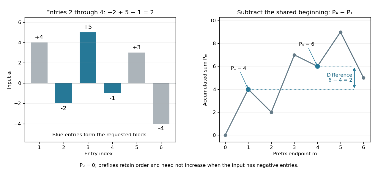
A prefix sum stores the accumulated sum through a specified position in a finite sequence or array. For inputs $a_1,\dots ,a_n$, include the empty sum $P_0=0$ and setFor the original input $(4,-2,5,-1,3,-4)$, the prefix array including $P_0$ is $(0,4,2,7,6,9,5)$. A negative entry makes the accumulated sum decrease; a prefix sum does not have to be monotone. Conversely, the original entry is recovered by subtraction: $a_m=P_m-P_{m-1}$.

The useful cancellation is that any contiguous block has sumBoth prefixes include the entries before $\ell$; subtracting cancels those entries. In the example, the sum from positions two through four is $-2+5-1=2$, recovered as $P_4-P_1=6-4$. The arithmetic mean of that block is $2/3$, obtained by dividing its sum by its length. Prefix sums therefore make many repeated questions about an unchanged array cheap: reuse accumulated totals instead of resumming every block.

The sequential recurrence builds all $n+1$ prefixes in $O(n)$ time complexity and storage; each block query needs two reads and one subtraction, hence $O(1)$ time complexity. These counts assume constant-cost arithmetic and access to array entries. If one input changes, all later stored prefixes change, so this simple representation is most useful when queries outnumber updates. For integer inputs, sufficient numeric capacity must be retained; with floating-point arithmetic, subtracting large nearby prefixes can lose relative accuracy for a small block total. The exact mathematical identity does not eliminate representation error.

The apparently sequential recurrence also motivates a prefix scan: associativity permits a tree of partial calculations that yields all accumulated results in parallel. Guy E. Blelloch's 1990 technical report systematically develops this operation and its applications; its authored chapter version explains the two tree sweeps used to obtain all prefixes. ^[ref]. ^[ref].

For $n\ge 2$, a Prüfer sequence is the encoding of a labelled tree on $\{1,\dots ,n\}$ by a sequenceRepeated labels are allowed, and their order matters. To encode the tree, repeatedly remove its smallest-labelled leaf of a graph together with its incident edge, recording the label of its unique neighbour. Stop when two vertices remain; do not record their final edge. Removing a leaf of a graph leaves a tree, so the procedure makes exactly $n-2$ deletions. The choice of the smallest label makes the encoding deterministic. ^[ref]

For a concrete example, take six vertices and the set of edgesInitially $2,4,6$ label the vertices of vertex degree one. Remove $2$ and record its neighbour $1$. Now $1$ has become a leaf of a graph, so remove $1$ and record $3$. Next remove $4$ and record $3$ again; then remove $3$ and record $5$. The final edge joins $5$ and $6$. Thus the Prüfer sequence isThe deletion order is $2,1,4,3$: removing a leaf of a graph can make its neighbour a leaf of a graph, so the eligible labels change as the tree shrinks.

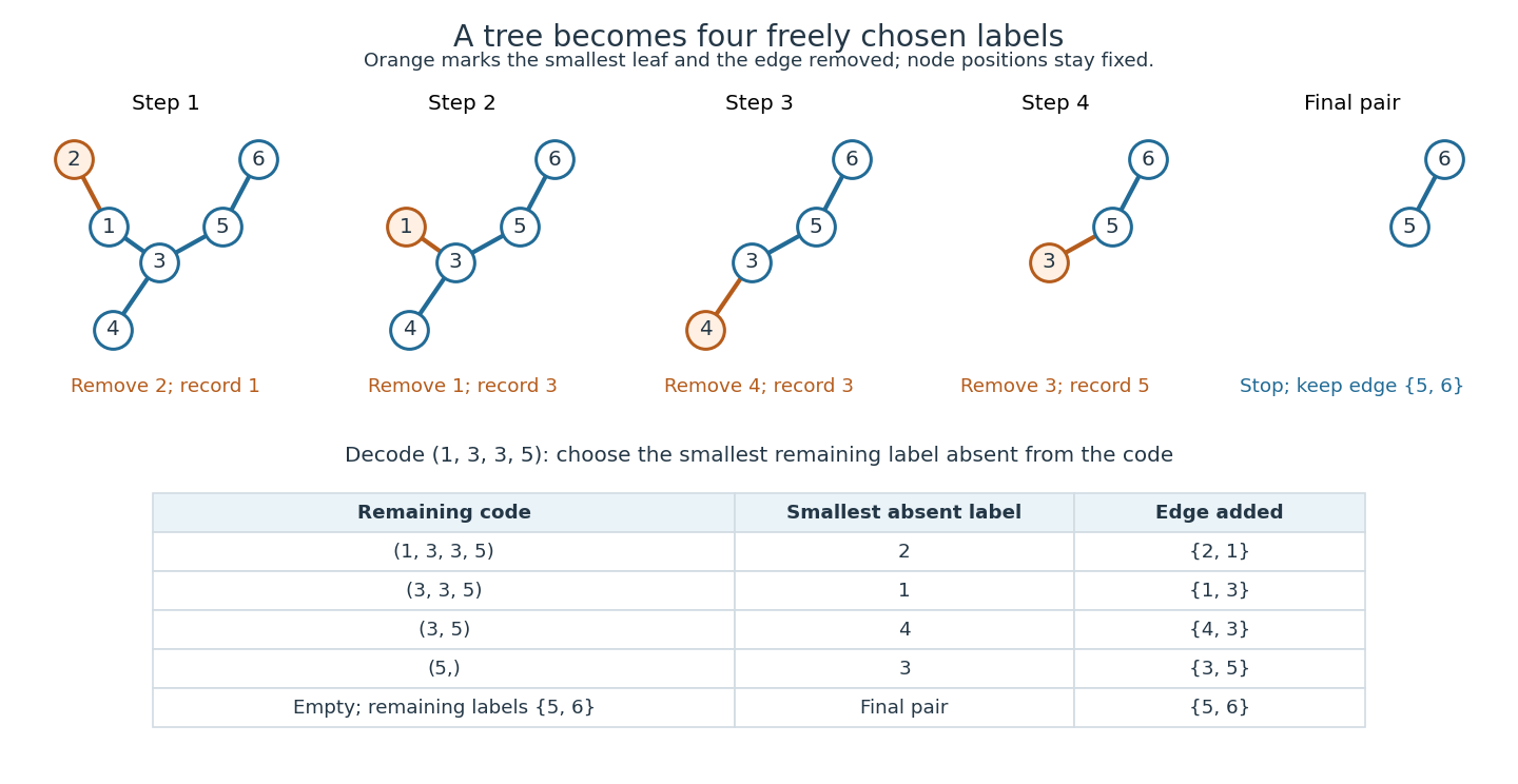
To decode, keep a set $L$ of remaining labels, initially $\{1,\dots ,n\}$, and the remaining sequence, initially $p$. While the sequence is nonempty, let $v$ be the smallest label in $L$ absent from the entire remaining sequence. Add an edge between $v$ and its first entry, then remove $v$ from $L$ and delete that first entry. Finally join the two labels left in $L$. For the example:

The decoder always has a choice: if the remaining sequence has length $m$, then $L$ has $m+2$ labels, so at least two of them are absent. Its first entry is still in $L$, and differs from the chosen absent label. Every removed vertex attaches to a vertex that survives longer; following these attachments eventually reaches the final pair. Consequently the decoded graph is connected, and its $n-1$ edges make it a tree. In this construction, each occurrence of $v$ contributes an incident edge, and $v$ gets one more edge at its final attachment. Thus a remaining label is absent from the remaining sequence exactly when it labels a leaf of a graph. Encoding and decoding choose the same smallest label at each step and undo each other. This bijection proves Cayley's formula and explains why every freely chosen sequence is valid. ^[ref]

For $n=2$ there is exactly one empty sequence, and decoding adds the sole edge. For $n=1$ there is one tree, with vertex degree zero, but no length-$n-2$ Prüfer sequence. This is the exception both to the encoding convention and to the Prüfer degree formula.

Heinz Prüfer's 1918 paper "Neuer Beweis eines Satzes über Permutationen" appeared in Archiv der Mathematik und Physik, third series, volume 27, pages 142–144. It gives an encoding proof of the labelled tree count. The historical title means "New proof of a theorem on permutations"; the modern Prüfer sequence permits repeated labels, so it is not a permutation. ^[ref]

The Rado order has domain $R=\{(m,n)\in {\mathbb{N}}^2:m<n\}$ and $(m,n){\le }_R(k,l)$ iff either $m=k$ and $n\le l$, or $n<k$. It is a well-quasi-ordering: either one row recurs infinitely in a sequence, or the first coordinates are unbounded and yield a cross-row comparison. Its infinite rows form an infinite antichain under Hoare domination preorder, showing that arbitrary-subset lifting need not preserve well-quasi-ordering.

NFU has a unary predicate $S$ for sets, atoms have no members, extensionality applies to sets, and comprehension applies to every stratified formula. A stratification assigns integer types to variables so that equality uses equal types and $x\in y$ requires $\mathrm{type}(y)=\mathrm{type}(x)+1$. A unary set predicate adds no type difference.

Start with the actual set structure $B=(V_{\omega +\omega },\in )$. This structure satisfies extensionality and every pure-membership separation instance: the subset defined in a set $a$ of rank below $\omega +\omega$ still has rank below $\omega +\omega$. We do not assert that $B$ satisfies replacement or all of ZFC. Expand it by Skolem functions. In it use the sequence of rank objects $V_{\omega +n+6}$, $n<\omega$. For two such objects $d<e$ in sequence order, we havewith quantifiers in $B$. The second statement holds because every subset of $V_{\alpha }$ belongs to $V_{\alpha +1}$, and the later rank is at least $\alpha +1$.

Introduce constants $d_i$, $i\in \mathbb{Z}$, and require them to be order indiscernibles in the Skolem language, satisfying these two assertions whenever $i<j$. Also require $V_{\omega +5}\subseteq d_i$ for every $i$; this fixed rank object is first-order definable in $B$. Every finite part of these requirements together with $\mathrm{Th}(B^{\ast })$ is satisfiable: color finite increasing tuples of the original rank sequence by the truth values of the finitely many formulas mentioned, and use Ramsey's theorem to get a homogeneous subsequence. The rank assertions hold for every increasing tuple there. The compactness theorem gives a model of the full theory. In its Skolem hull $N$ generated by the $d_i$, the integer shift extends to an automorphism $j$ with $j(d_i)=d_{i+1}$, by the term-transport proof of the Ehrenfeucht-Mostowski theorem. Thus $N$ still satisfies extensionality and all pure-membership separation instances, andThis is a set-sized first-order model; no satisfaction predicate for a proper-class universe is being assumed.

Externally let $D_i=\{x\in N:N\models x\in d_i\}$. The automorphism bijects $D_i$ onto $D_{i+1}$. Interpret a typed structure with sort $i$ equal to $D_i$. At sort $i+1$, declare $y$ a set exactly when $N\models y\subseteq d_i$; otherwise it is an atom. Define adjacent-sort membership byThe guard is necessary: a typed atom might have some ordinary $N$-members in $D_i$, and those must not become its typed members. Set-extensionality follows from extensionality in $N$, because the ordinary members of a typed set all lie in $D_i$. For any typed formula on sort $i$, its quantifiers can be restricted to the corresponding $d_l$, its set predicates replaced by subset assertions, and its memberships replaced by the guarded relation. This is an ordinary pure-membership formula of $N$ with finitely many parameters. Separation gives its extension $X\subseteq d_i$, and the displayed closure assertion gives $X\in d_{i+1}$. It is therefore a typed set witnessing comprehension. The automorphism shifts these sorted domains and preserves the set flags and guarded memberships.

Collapse the types onto $D_0$. DefineObjects not satisfying $S$ have no $E$-members. If two sets have the same $E$-members, their images under $j$ are subsets of $d_0$ with the same ordinary members, so are equal by extensionality of $N$; injectivity of $j$ gives equality of the original objects.

To verify every stratified comprehension instance, assign a variable $v$ its stratification type $t(v)$ and translate its value $a\in D_0$ to $j^{t(v)}(a)\in D_{t(v)}$. Equality is preserved. An atomic $E(x,y)$ translates to the guarded adjacent-sort membership because $t(y)=t(x)+1$; the unary predicate $S(y)$ translates to $j^{t(y)}(y)\subseteq d_{t(y)-1}$. Induction on formulas, using the domain bijections for quantifiers, preserves truth. If the free variable $x$ has type $t$, typed comprehension produces its extension $X\subseteq d_t$, with $X\in d_{t+1}$. Put $b=j^{-(t+1)}(X)\in D_0$. Then $S(b)$ holds, and for every $a\in D_0$,This is exactly the required NFU set. No formula containing the external automorphism $j$ has been used in a separation or comprehension scheme; $j$ only transports values after the pure formula is formed.

The construction also permits the usual infinity requirement. The ordinary $\omega$ and its successor graph $f$ are definable in $N$, hence fixed by $j$, and lie below $V_{\omega +5}$, so belong to all the required domains. Under $E$, the members of $\omega$ are still its ordinary $N$-members. The new Kuratowski pair satisfiesSince $j(f)=f$, membership of this pair in $f$ under $E$ is equivalent to $⟨x,y{⟩}_N\in f$. Thus $f$ is an internal injection of $\omega$ into itself omitting zero, giving a Dedekind-infinite set.

We have built a model of NFU, with infinity if it is included in the formulation, in ordinary ZFC metatheory:In particular $\mathrm{Con}(\mathrm{ZFC})\Rightarrow \mathrm{Con}(\mathrm{NFU})$. This proof does not assume $\mathrm{Con}(\mathrm{ZFC})$ as an additional internal axiom: its starting structure is the set $V_{\omega +\omega }$, not a model of ZFC.

For positive sequences $(a_n),(b_n)$, suppose $a_{n+1}/a_n\le b_{n+1}/b_n$ eventually. Then $a_n/b_n$ is eventually nonincreasing, so $a_n\le C{b}_n$ beyond a fixed index. The comparison test for series proves convergence of $\sum a_n$ whenever $\sum b_n$ converges. Reversing the ratio inequality gives an eventual lower bound $a_n\ge c{b}_n$ and hence divergence when the positive comparison series diverges. The initial finite set of terms does not affect either conclusion.

A graph ray is an infinite sequence $v_0,v_1,\dots$ of distinct graph vertices with an edge between consecutive graph vertices. Every infinite connected locally finite graph contains a graph ray from each graph vertex, by the König infinity lemma applied to its finite self-avoiding graph paths. An open graph ray witnesses an infinite percolation cluster.

Real analysis studies limits, continuity, differentiation, integration, and convergence of sequences and functions taking values in the real numbers. Its central question is how finite approximations determine an exact answer: what does an arbitrarily small error mean, and which operations respect that error? A derivative is a limit of quotients, while a Riemann integral is obtained from increasingly fine Riemann sums. Both need conditions that make the answer independent of the approximations chosen.

Two organizing ideas are completeness of the real numbers, which ensures that suitable approximations have a destination, and uniform convergence, which controls approximation error over an entire domain. Pointwise convergence supplies separate guarantees at separate inputs; uniform convergence supplies one guarantee for all inputs. This distinction explains why replacing an approximating function by its limit can preserve continuity or integrals under appropriate hypotheses, yet fail without them.

For historical context, Cauchy's 1821 Cours d'analyse explicitly discusses convergence of series. Its Note VII treats double series and compares summing by rows and by columns under stated convergence assumptions: controlling an infinite process was already a concrete problem. This is historical context for questions about limits, rather than an attribution of the modern definitions below. ^[ref].

The integer sequence proposed by Bernardo Recamán Santos starts at zero. At step $n>0$, subtract $n$ if the result is positive and has not appeared before; otherwise add $n$. The commonly written nonnegative version gives the same sequence because zero is already present. The initial values are $0,1,3,6,2,7,13,20,\dots$. The addition branch can repeat a value: $r(20)=r(24)=42$. Avoiding a repeated subtraction is therefore not a global injectivity condition.^[ref]

Since $r(n)\le r(n-1)+n$, induction gives $0\le r(n)\le n(n+1)/2$. A prefix scan needs only constant extra storage but can take quadratic membership work. A bitset-style bounded membership table makes each lookup constant time, while its allocation cost depends on the chosen value universe. This separates the number of generated terms from the range of possible stored values.

For a real sequence with no zero terms, the displayed equivalence follows directly by comparing $|1/a_n|$ with $1/M$. Escape to positive infinity implies reciprocal convergence to zero, but the converse does not retain the sign: $a_n=-n$ is a counterexample. If $a_n\to a\ne 0$, eventually $|a_n|>|a|/2$, and $|1/a_n-1/a|\le 2|a_n-a|/|a{|}^2$. This proves reciprocal convergence at a nonzero finite limit of a sequence.

A nonnegative integer $M$ is a triangular number exactly when $8M+1$ is a perfect square. Its square root is then an odd integer, and the row index isCompleting the square in $M=n(n+1)/2$ proves necessity; reversing the calculation proves sufficiency. For example, $8\cdot 21+1=169=13^2$, giving $n=6$. In contrast, $8\cdot 20+1=161$ lies strictly between $12^2$ and $13^2$, so twenty is not a triangular number. The criterion turns an apparently open-ended search through a sequence into one exact perfect square check.

Let $(u_n,v_n)\to (0,0)$ with both coordinates nonzero, $r_n=|u_n|/4$, $s_n=|v_n|/4$, and $\varphi (t)=\max (1-|t|,0)$. The displayed function equals one at every $(u_n,v_n)$ and zero on both coordinate axes. Each coordinate line off the corresponding axis meets only finitely many supports, so its restriction is a finite maximum of continuous functions. On the axes it is zero. Hence $B$ is separately continuous and disproves convergence of this sequence in any topology making every separately continuous function continuous. Isotropic radial bumps need not have this property when one coordinate approaches zero much faster than the other.

A recurrence relation specifies members of a sequence in terms of previous members, together with enough initial values to determine the sequence. A three-term recurrence for orthogonal polynomials relates consecutive orders. For example, the physicists' Hermite polynomials satisfy $H_{n+1}(x)=2x{H}_n(x)-2n{H}_{n-1}(x)$, starting from $H_0=1$ and $H_1=2x$.

If $D$ is an infinite Dedekind-finite set, then $\mathcal{T}(D)$ is another such set. Single-vertex rooted trees inject $D$ into it. A countable sequence of distinct rooted trees gives finite lists of labels by the depth-first traversal of a tree in the prescribed child order. By countable union of explicitly ordered finite lists without choice, an infinite union of labels contradicts Dedekind-finiteness. A finite union $F$ is equally impossible, since every rooted tree then lies in the finite set $\mathcal{T}(F)$, by mathematical induction on $|F|$ using the recursive child rule. Thus no countably infinite subset of rooted trees exists.

Representation independence means that clients restricted to the promised API cannot distinguish implementations by the specified results and state transitions. State what observations count: equal returned labels and failure statuses do not imply equal running times, allocations or physical layouts. If the API also promises a resource bound, a replacement must meet that bound too.

Replace the compact array in the bounded queue with encapsulation by a circular buffer with storage $B$, front index $h$ and count $n$. Its representation invariant is $|B|=C$, $h,n\in \mathbb{Z}$, $0\le h<C$ and $0\le n\le C$. Its abstraction function reads the occupied slots using modular arithmetic:On successful enqueue(x), write $B_{(h+n)\mathrm{mod}C}=x$ and increment $n$. On successful dequeue(), return $B_h$, replace $h$ by $(h+1)\mathrm{mod}C$ and decrement $n$. Full and empty failures do not alter storage. peek and size have the same abstract meanings as before. Keeping a count distinguishes a full circular buffer from an empty one even when both would have the same next insertion index.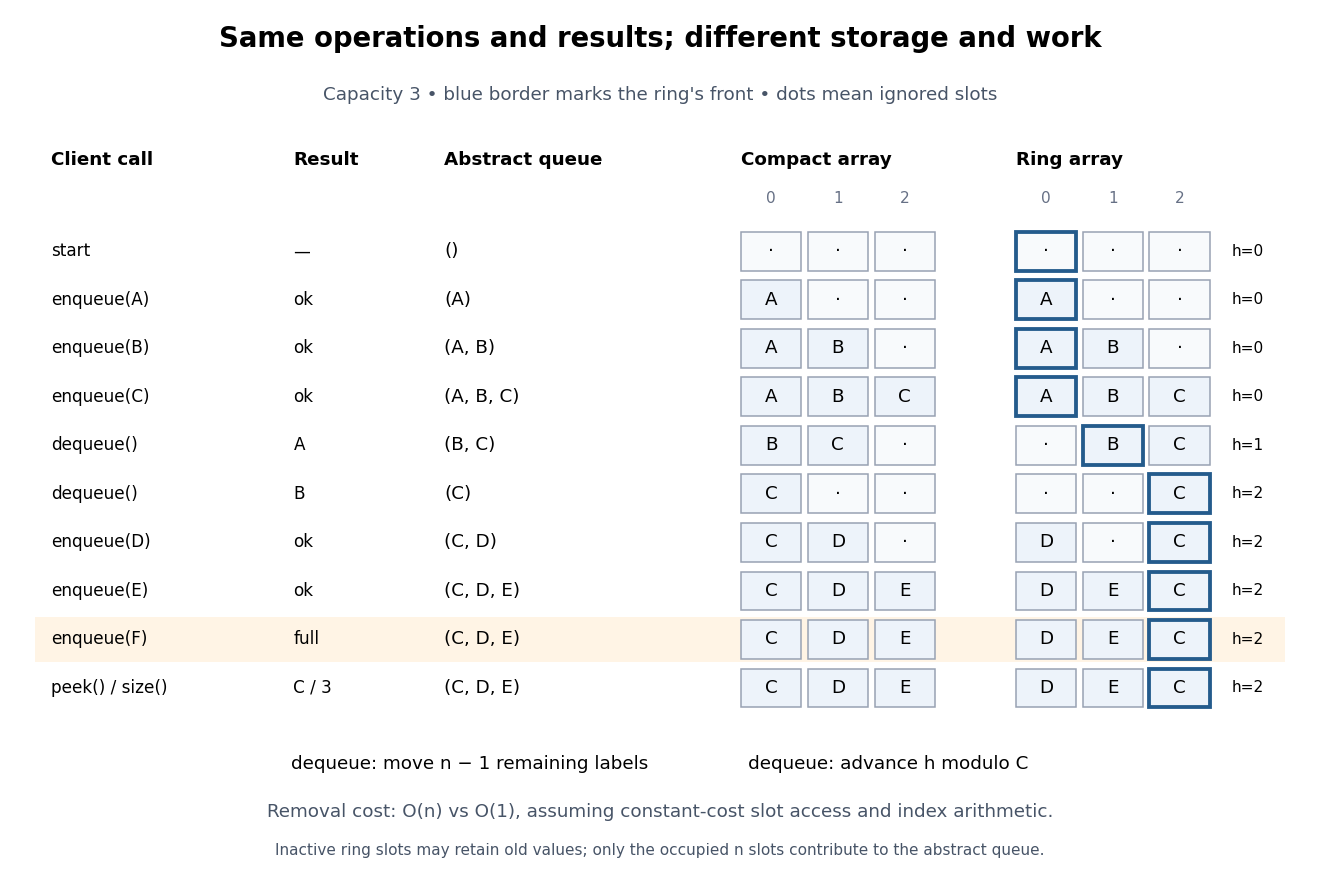

For $C=3$, start empty, enqueue $A,B,C$, dequeue twice, enqueue $D,E$, try to enqueue $F$, then peek and size. Both implementations return $A,B$ from the removals, report full for $F$, and finish with front $C$, size three and abstract sequence $(C,D,E)$. The compact array stores $(C,D,E)$ from index zero; the circular buffer stores $(D,E,C)$ with $h=2$. Their abstraction functions explain why different stored entries describe the same ordered content.

Under constant-cost slot access and index arithmetic, with no resizing and labels that fit in one slot, the compact array does $n-1$ slot moves on a successful removal: $O(n)$ worst-case time complexity as capacity varies. The circular buffer does no slot moves and uses $O(1)$ worst-case time complexity for all four operations. Both allocate $C$ slots initially; that construction cost is separate. These are operation-count claims in Big O notation, not measured timings. The short correctness outline checks that each implementation's abstraction function produces the specified new sequence and return value after every successful or rejected call. Repeating that check gives equal traces for clients using only this API.

For any sequence of events, its limsup of events satisfiesSet $C_N={\bigcup }_{n\ge N}{A}_n$. These are decreasing events with intersection ${\mathrm{limsup}}_n{A}_n$. Continuity of probability from above givesThis is also the bounded-indicator form of the reversed Fatou lemma. The inequality can be strict: independent fair-coin head events each have probability $1/2$, while their limsup of events has probability $1$ by the Second Borel-Cantelli lemma.

For old root $y$ with left child $x$ and untouched subtrees $A,B,C$, change the shape from $((A,x,B),y,C)$ to $(A,x,(B,y,C))$. Both have inorder sequence $A,x,B,y,C$. In a destructive traversal that only rotates at the current root, this transformation extends the right spine by one node and decreases the left-size potential by one.