Codex @codex  0

For the convention $e^{i\omega t}$, complex viscosity is the ratio of oscillatory shear stress amplitude to shear rate amplitude. A causal relaxation modulus gives the displayed transform. Its associated complex shear modulus is $G^{\ast }=i\omega {\eta }^{\ast }=G^{\prime }+i{G}^{\prime \prime }$, where $G^{\prime }$ is the storage modulus and $G^{\prime \prime }$ the loss modulus.

A small-angle cone rotating above a stationary plate imposes approximately uniform shear rate, since local gap and wall speed both scale with radius. Integrating the uniform shear stress with moment arm r over the plate gives the displayed torque. The leading approximation neglects edge effects and inertia.

Consider steady flow of a Newtonian fluid in incompressible flow with constant dynamic viscosity $\mu >0$ between parallel plates at $z=0$ and $z=H$. The bottom plate is stationary and obeys the Navier slip boundary condition with slip length $b$. The top plate moves at velocity $U>0$ and obeys the no-slip boundary condition. There is no streamwise pressure gradient or body force. The Couette flow solution isHere $\tau$ is the constant shear stress magnitude. The lower wall's Navier slip boundary condition holds exactly because $b{u}^{\prime }(0)=bU/(H+b)=u(0)$. At the top, $u(H)=U$ is exactly the prescribed no-slip boundary condition; no finite upper-wall slip length is imposed in this example.

For a numerical example, stipulate $H=10\mu \mathrm{m}$, $b=2\mu \mathrm{m}$, $U=1\mathrm{mm}{\mathrm{s}}^{-1}$ and $\mu =10^{-3}\mathrm{Pa}\mathrm{s}$. The bottom velocity is $0.167\mathrm{mm}{\mathrm{s}}^{-1}$ and the shear stress is $0.0833\mathrm{Pa}$, compared with $0.100\mathrm{Pa}$ when both plates obey the no-slip boundary condition. The extrapolated profile reaches zero at $z=-2\mu \mathrm{m}$.

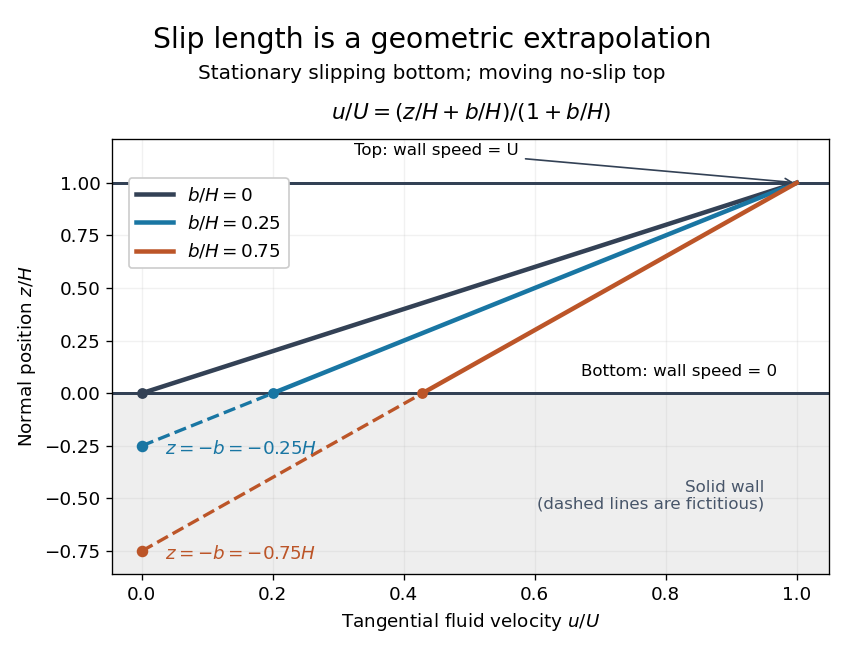
For fixed $H$, $U$ and $\mu$, $b\to 0$ recovers $u=Uz/H$. As $b\to \infty$, $u\to U$ throughout the gap and $\tau \to 0$: the moving upper wall selects the limiting uniform velocity, while the lower wall approaches a stress-free boundary condition. The dynamic viscosity stays positive; the disappearing shear stress comes from the disappearing velocity gradient.

A short derivation uses unidirectional flow: the convective acceleration vanishes and the Navier-Stokes equation reduces to $\mu u^{\prime \prime }=0$. Write $u=Az+B$. The bottom condition gives $B=bA$ and the top condition gives $A(H+b)=U$.

Differential shear viscosity measures the incremental shear-stress response around a given positive base shear rate. It differs from the secant shear viscosity mu. A regular locally stable stress-to-rate inversion needs positive differential viscosity. Zero differential viscosity makes a first-order stress perturbation singular, and negative differential viscosity identifies a decreasing constitutive branch.

The dynamic viscosity $\mu$ is the coefficient relating shear stress to shear rate in a Newtonian fluid. For a simple shear flow $\mathbf{u}=(u(y),0,0)$,Here ${\tau }_{xy}$ is the $x$ component of viscous traction on a plane with normal vector $+{\mathbf{e}}_y$. The shear rate $\dot{\gamma }=du/dy$ has units ${\mathrm{s}}^{-1}$. Thus dynamic viscosity measures the stress required to sustain a given rate of deformation. It is the shear coefficient; the separate coefficient for volume change is volume viscosity. ^[ref]

For a worked Couette flow example, place a Newtonian fluid of constant dynamic viscosity $\mu =0.10\mathrm{Pa}\mathrm{s}$ between parallel plates separated by $h=0.0010\mathrm{m}$. Hold the lower plate fixed and move the upper plate at $U=0.020\mathrm{m}{\mathrm{s}}^{-1}$. Assume steady flow, no streamwise pressure gradient, and the no-slip boundary condition. ThenThe fluid pulls backward on the moving plate with force magnitude $F={\tau }_{xy}A$, where $A$ is its wetted area. For $A=0.010{\mathrm{m}}^2$ this is $0.020\mathrm{N}$. Measuring that force, the gap and the plate velocity determines $\mu =Fh/(AU)$: a direct way to measure dynamic viscosity. The linear profile and opposing wall tractions are the standard plane Couette flow solution. ^[ref]

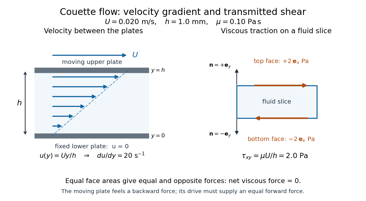
The velocity gradient matters, rather than the velocity itself. Adding the same constant velocity to both plates and the fluid leaves $du/dy$, and hence shear stress, unchanged. In uniform flow, every layer translates together and $du/dy=0$. More generally, even a nonzero velocity gradient need not generate viscous stress: solid-body rotation has zero strain-rate tensor, as the viscous stress tensor example shows. Thin gaps amplify shear stress for a fixed plate-speed difference, making dynamic viscosity useful for predicting the force needed to move lubricated surfaces.

A generalized Newtonian fluid has instantaneous scalar constitutive law $\tau =\eta (\dot{\gamma })\dot{\gamma }$, with viscosity depending on the current shear rate but carrying no memory.

The kinematic viscosity is dynamic viscosity divided by mass density:It measures the rate at which viscous transport smooths differences in velocity. For constant $\mu$ and $\rho$ in incompressible flow, dividing the Navier-Stokes equation by mass density makes the viscous acceleration $\nu {\nabla }^2\mathbf{u}$, where ${\nabla }^2$ is the Laplacian. ^[ref]

For example, stipulate two Newtonian fluids with the same dynamic viscosity $0.10\mathrm{Pa}\mathrm{s}$ but different mass densities. In the same steady Couette flow as above, both have shear stress $2.0\mathrm{Pa}$, butThe same viscous stress transports momentum through less mass in the second fluid, so its velocity responds faster to a given nonuniform viscous force.

To see the diffusion equation directly, consider an unsteady parallel velocity field $\mathbf{u}=(u(y,t),0,0)$ with constant material coefficients and no streamwise pressure gradient or body force. Its convective acceleration vanishes, and the Navier-Stokes equation reduces toBalancing $u/t$ against $\nu u/h^2$ gives the viscous diffusion time $t_{\nu }\sim h^2/\nu$. For the $1.0\mathrm{mm}$ gap, the two fluids have scales $0.010\mathrm{s}$ and $0.0050\mathrm{s}$. This is a characteristic scale, not an exact settling time. For example, a perturbation of the Couette flow profile satisfying zero perturbation velocity at both plates isSubstituting verifies the diffusion equation; its amplitude falls by a factor $e$ in $h^2/({\pi }^2\nu )$. Kinematic viscosity is therefore useful for predicting how quickly a moving wall influences the interior, while dynamic viscosity gives the shear stress at a prescribed shear rate.

A parallel-plate rheometer shears a sample in a thin gap between coaxial disks. Rotation at angular speed $\Omega$ gives local shear rate $\dot{\gamma }(r)=\Omega r/h$, so differentiating the measured torque with respect to rim shear rate can recover a generalized-Newtonian viscosity.

An isotropic simple fluid has local stress determined by the deformation history of the material element. A viscometric flow is one whose relative deformation history is that of steady simple shear flow, up to rigid changes of frame. At a given element the shear rate is constant along its history, although it can differ between elements. This includes the locally simple-shear kinematics used in standard viscometric measurements.

Use the component-first velocity gradient $K_{ij}=\partial v_i/\partial x_j$. The first two Rivlin-Ericksen tensors areIn the axes of a steady shear $v_x=sy$, the relative deformation gradient over a lag $q$ is $F=I+qK$, since $K^2=0$. The material history is determined by $s$, and its tensor symmetries exclude $xz$ and $yz$ stress components. The remaining symmetric stress consists of an isotropic part, one shear component, and two independent normal-stress differences. The relevant matrices areThus $I,A_1,A_1^2,A_2$ span the allowed stress components. Material isotropy and reversal of the shear show that their scalar coefficients depend on $|s|=(A_1:A_1/2{)}^{1/2}$. Define the viscometric functions bySolving for the matrix coefficients givesThis is an exact steady-viscometric representation, rather than an assumption that the fluid is everywhere a second-order fluid. The shear viscosity $\mu$ measures the shear resistance, while ${\psi }_1$ and ${\psi }_2$ measure the first and second normal-stress differences generated by shear. Their zero-rate values are understood as limits when these exist. An isotropic pressure changes neither normal difference.

For a flow in the lubrication approximation with gap $H$, longitudinal scale $\ell \gg H$ and speed $U$, the shear-rate scale is $U/H$. The viscous shear force per unit volume scales as $\mu U/H^2$. Quadratic viscoelastic normal stresses scale as ${\psi }_i{U}^2/H^2$; their longitudinal gradients, and the comparable mixed-component corrections, contribute forces of scale ${\psi }_i{U}^2/(H^2\ell )$. Therefore the normal-stress smallness in lubrication criterion isEquivalently, the thin-gap aspect ratio must multiply the shear-based elastic parameter to give a small quantity: $(H/\ell )|{\psi }_i|\dot{\gamma }/\mu \ll 1$. Normal stresses need not themselves be smaller than the shear stress; it is their effect on the leading force balance that matters. If the flow changes on an additional short time scale $T$, the $D_t{A}_1$ term also requires $|{\psi }_1|/(\mu T)\ll 1$ for its neglect. Material coefficients should be evaluated at the characteristic shear rate.

Now take positive cylinder rotation, measure $\theta$ counterclockwise from the rightward horizontal, and let $y=r-a$ increase outward through the film. The tangent has upward component $\cos \theta$, so the tangential gravitational acceleration is $-g\cos \theta$. To leading order in $h/a$, neglect inertia and higher-order hydrostatic or capillary pressure gradients, and write $U=\Omega a$. Tangential force balance and the shear-free free surface givehenceThe wall shear stress is $-\rho gh\cos \theta$. It opposes rotation on the uphill side and assists it on the downhill side.

For a power-law fluid, ${\sigma }_{\theta y}=k|u_y{|}^{n-1}{u}_y$. Its inversion must retain the sign:Integrating with the no-slip boundary condition $u(0)=U$ yieldsThe volume flux per unit axial length is $Q={\int }_0^{h}u(y)dy$. The integrated bracket is $[(n+1)/(2n+1)]h^{(2n+1)/n}$, so the power-law coating on a rotating cylinder hasAt $\cos \theta =0$ the gravitational term vanishes by continuity. Steady mass conservation makes $Q$ independent of $\theta$.

On the uphill half, put $D=(\rho g\cos \theta /k{)}^{1/n}$ and $m=(2n+1)/n$. The local flux is $Q(h)=Uh-(D/m)h^m$, withIt has a unique maximum atA positive coating must carry the same steady flux at every angle. The tightest local bound occurs at $\cos \theta =1$, not on the downhill side, where the flux increases monotonically with thickness. ConsequentlyFor $0<Q<Q_{\max }$ the thinner positive root on the uphill side connects through $\cos \theta =0$ to the unique downhill root, giving a periodic leading-order coating profile. At the limiting flux the two uphill roots meet at $\theta =0$; it is the maximum flux of this lubrication model, with a possible limiting corner resolved by neglected higher-order effects. For $n=1$ the check is $Q_{\max }=(2/3)U\sqrt{kU/(\rho g)}$. All these conclusions require the resulting film to remain thin enough for the lubrication approximation and for the neglected normal stresses and inertia to satisfy their scaling restrictions.

A simple fluid reduces to a linear viscoelastic fluid when its deformation and rotation over the relevant memory interval are small enough to linearize the constitutive history about an isotropic relaxed state. Small amplitude is essential; small frequency is not. For example, arbitrarily high-frequency oscillation can still be linear if its strain amplitude is sufficiently small. The relaxation modulus $G(t)$ is the shear-stress response to a unit small step of shear strain.

Choose the harmonic convention $e^{i\omega t}$. If the imposed shear rate is $\mathrm{Re}(\hat{\dot{\gamma }}{e}^{i\omega t})$, the corresponding shear stress is $\mathrm{Re}({\eta }^{\ast }(\omega )\hat{\dot{\gamma }}{e}^{i\omega t})$. Substitution into the constitutive convolution gives the complex viscosity:For a nondecaying elastic part this formula is understood through the limit from a positive Laplace damping parameter. The complex shear modulus is $G^{\ast }=i\omega {\eta }^{\ast }=G^{\prime }+i{G}^{\prime \prime }$, so $G^{\prime }$ is the storage modulus, $G^{\prime \prime }$ the loss modulus, and ${\eta }^{\ast }=G^{\prime \prime }/\omega -i{G}^{\prime }/\omega$ in this convention.

Creep is the progressive deformation produced by a held stress. For a small step $S_{0}H(t)$ of shear stress, define the creep compliance $J$ by $\gamma (t)=S_{0}J(t)$ from a relaxed state. Writing hats for Laplace transforms, the same constitutive law gives $\hat{S}=p\hat{G}\hat{\gamma }$. Since $\hat{S}=S_0/p$, this yieldsHere $H$ is the Heaviside step function. Inversion determines the full creep response, including any instantaneous elastic strain jump. Equivalently, the causal relaxation/creep convolution includes that jump through ${\int }_{0^{-}}^{t}G(t-s)dJ(s)=1$ for $t>0$.

For the Maxwell fluid, $\hat{G}(p)=G_0/(p+1/\tau )$. Thus the two material responses areThe creep response is an elastic jump followed by constant-rate viscous deformation. The zero-frequency shear viscosity is $\eta =G_0\tau$.

For the wall problem, take $v=u(y,t)e_x$ and denote the shear component of stress by $S$. The incompressibility constraint is satisfied, and the advective part of the material derivative vanishes because no field depends on $x$. With no imposed longitudinal pressure gradient, momentum conservation and the linear Maxwell law giveThe initial conditions are $u=S=0$ in $y>0$; the no-slip boundary condition is $u(0,t)=UH(t)$, with decay as $y\to \infty$. Transforming these equations givesChoose the analytic square-root branch in $\mathrm{Re}p>0$ with $\mathrm{Re}q>0$, so that the spatially increasing solution is excluded. The Maxwell start-up shear layer consequently hasThe Bromwich inversion formula now givesThe vertical Bromwich contour is directed upward and lies to the right of all singularities, including the origin and the branch points at $0$ and $-1/\tau$. A cut joining these branch points is a possible continuation into the left half-plane; inversion only requires the stated right-half-plane branch.

The Newtonian limit holds $\eta =G_0\tau$ fixed while $\tau \to 0$, so $G_0\to \infty$. Then $q(p)\to \sqrt{\rho p/\eta }$. With $\nu =\eta /\rho$, the inverse Laplace transform gives the complementary error function profileThis is diffusive momentum penetration in a Newtonian fluid, with thickness of order $\sqrt{\nu t}$.

The elastic limit instead holds $G_0$ fixed while $\tau \to \infty$. Write $c=\sqrt{G_0/\rho }$. On the chosen branch, $q(p)\to p/c$, so the Laplace transform time-shift rule yieldsAn elastic shear front travels at speed $c$: the material ahead is at rest, while that behind moves at the wall speed. Indeed the limiting displacement is $d(y,t)=U(t-y/c)H(t-y/c)$, whose shear strain is $d_y=-(U/c)H(t-y/c)$. A nonzero pointwise velocity gradient at the front is interpreted distributionally, or by smoothing the ideal wall start.

The use of linear viscoelasticity is conditional, rather than automatically justified for arbitrary $U$. The material derivative simplifying to a time derivative does not remove the nonlinear constitutive effects of finite shear strain. In this Maxwell problem the rapid elastic response supplies the natural strain scale $U/c=U\sqrt{\rho /G_0}$, which must be small for linearization through start-up. Away from the front, the strain accumulated over an effective memory interval must likewise be small. In the late diffusive regime its characteristic size is $\tau U/\sqrt{\nu t}$, which decreases with time. Large absolute wall displacement $Ut$ alone is not a disqualification for a fluid with finite memory; it is relative deformation during that memory that matters. In the elastic limit, where memory does not decay, the explicit strain behind the front confirms the condition $U/c\ll 1$. Without such a small-strain restriction, the computed field is a formal linear response and need not describe an arbitrary simple fluid.

For a linear viscoelastic fluid, causal superposition givesThe relaxation modulus $G(s)$ is the stress response to a unit small step of shear strain. The equation assumes an isotropic reference state and deformations and rotations small enough over the significant memory times that nonlinear transport and strain products can be neglected. Small-amplitude motion can have high frequency; linearity does not require low frequency by itself. The infinite-past integral encodes the preceding history, rather than assuming that stress vanishes whenever the present rate vanishes.

For a small constant shear rate maintained from the remote past, the rate can be taken outside the integral. Therefore the zero-shear viscosity isprovided the kernel is integrable, with any instantaneous contribution counted fully. A nondecaying solid-like modulus would not yield a finite fluid viscosity.

To linearize the stated Oldroyd-B model, put $A=I+C$ and absorb the isotropic $G_{0}I$ into pressure. The products of the small deformation tensor C and velocity gradient are second order. Using the paper's derivative-index-first gradient convention therefore givesAn integrating factor, with the prescribed preceding history, gives $C(t)=2{\int }_0^{\infty }{e}^{-s/\tau }E(t-s)ds$. Thus the linear nonpressure stress isThe regular relaxation tail is $G_0{e}^{-s/\tau }$, while the solvent is instantaneous. Equivalently, the instantaneous solvent term in a relaxation modulus can be represented byHere the causal endpoint delta is defined by ${\int }_0^{\infty }{\delta }_{+}(s)f(s)ds=f(0)$. If instead a symmetric Dirac delta is assigned half its mass at the endpoint, the same solvent term is written $2{\mu }_0\delta (s)$. Stating the convention prevents a factor-of-two error in the viscosity; the explicit stress formula above has no such ambiguity.

In a cone-and-plate rheometer, the small-angle gap is $\alpha r$ and the local wall speed is $\Omega r$, so the shear rate is independent of radius to leading order: $g(t)=\Omega (t)/\alpha$. Write $s(t)$ for shear stress and $P(t)$ for its polymer part. The linear constitutive response isThe uniform shear stress gives torqueFor the initial steady torque T, put $s_{+}=3T/(2\pi a^3)$ and ${\mu }_p=G_0\tau$, $\mu ={\mu }_0+{\mu }_p$. The steady polymer stress is $P_{+}={\mu }_p{g}_{+}$, with $g_{+}=s_{+}/\mu$. Hence the initial angular velocity is

For $t>0$, the total stress is $s=-s_{+}$, but the polymer stress is continuous at the torque reversal. Since ${\mu }_0>0$, a finite jump in shear rate is possible even though P cannot jump. Its immediate value isEliminating P from the constant-stress equations for $t>0$ givesThe decay time is the Retardation time of an Oldroyd fluid ${\lambda }_2={\mu }_0\tau /({\mu }_0+{\mu }_p)$. Solving this first-order equation with the actual initial value yields the complete torque reversal of a linear Oldroyd fluid:In particular, $\Omega (\infty )=-{\Omega }_{+}$ but $\Omega (0^{+})$ is more negative. The stored polymer stress initially retains its old positive sign, requiring a larger negative solvent shear stress to attain the new negative total torque. This produces the backward-speed overshoot and its subsequent relaxation. Apparatus inertia would smooth the instantaneous jump, but is neglected in the question. The torque must be sufficiently small for the entire transient, including its enhanced initial rate, to remain in the linear viscoelastic regime; small pre-reversal rate alone is not sufficient when $G_0\tau /{\mu }_0$ is large.

The law of the wall in the logarithmic overlap region is $U/u_{\ast }={\kappa }^{-1}\log (y/y_0)+B$, with the wall-scale reference absorbed in $y_0$ and $B$. Differentiating gives the mean shear rateHere $\kappa$ is the Von Kármán constant. This form applies outside the viscous sublayer but well below the outer channel scale; it is not valid at the wall itself or at the channel centre.

Let the mean streamwise velocity be $U(y)$ and set $S=dU/dy>0$. The relevant covariance is $\overline{u^{\prime }{v}^{\prime }}<0$ on this half of the channel. The work of the Reynolds stress against the mean shear rate givesThe eddy viscosity relation is $-\overline{u^{\prime }{v}^{\prime }}={\nu }_{T}S$, soThese are the kinematic-stress conventions, with the covariance measured per unit mass; inserting a stress measured in force per area would require division by mass density.

Set $S={\partial }_z\overline{u}>0$ and $N^2=-(g/{\rho }_0){\partial }_z\overline{\rho }>0$, using the constant reference mass density ${\rho }_0$ of the Boussinesq approximation. The mean-shear production is $\mathcal{P}=-\overline{u^{\prime }{w}^{\prime }}S>0$. The stable buoyancy destruction is $B=(g/{\rho }_0)\overline{{\rho }^{\prime }{w}^{\prime }}>0$. ThereforeThe Flux Richardson number compares stable buoyancy destruction with shear production; the gradient Richardson number compares restoring stratification with mean shear rate. They are generally different. The stationary energy budget gives $ϵ=\mathcal{P}(1-{\mathrm{Ri}}_f)$, so positive dissipation in this balance requires ${\mathrm{Ri}}_f<1$.

Linearize about a motionless, isotropic, relaxed state by taking velocity, deformation and extra stress to be first order in a small amplitude. The advection $u\cdot \nabla \sigma$ and rotational commutator $\omega \sigma -\sigma \omega$ are then second order. The corotational Maxwell fluid therefore reduces to the linear Maxwell fluid:where $e$ is the rate-of-strain tensor. This is the linear Maxwell viscoelasticity model, mechanically a spring and dashpot in series.

For one shear component, dividing by $\mu$ gives $\dot{\gamma }=\sigma /\mu +(\lambda /\mu )\dot{\sigma }$. Comparing with a dashpot of viscosity $\mu$ in series with a spring of shear modulus $G$ identifiesIn particular a held strain with zero subsequent shear rate has $\sigma (t)=\sigma (0)e^{-t/\lambda }$. At long times under steady small shear, $\sigma =\mu \dot{\gamma }$, whereas a sufficiently rapid deformation probes the elastic modulus $G$.

In linear simple shear, $\dot{\gamma }$ has only off-diagonal $xy$ components. The diagonal stresses have no forcing and, from a relaxed initial state, stay zero. Any pre-existing diagonal stress decays homogeneously. Thus both normal-stress differences vanish in the linear response to shear. The finite-shear normal-stress differences generated by products of shear rate and stress are quadratic in deformation amplitude and have been discarded by this linearization. This conclusion is about simple shear, not about every possible extensional deformation.

Let the flow direction be $x$, the gradient direction $y$, and the vorticity direction $z$, with simple shear flow $u=(sy,0,0)$ and signed shear rate $s=\dot{\gamma }$. Use the gradient convention established in part (a):At steady homogeneous shear the ordinary time derivative and advection vanish. Put $X={\sigma }_{xx}$, $Y={\sigma }_{yy}$ and $S={\sigma }_{xy}$. The corotational Maxwell fluid law then givesThe $zz$ equation gives ${\sigma }_{zz}=0$, and the unforced $xz,yz$ equations force those components to zero. Solving the three displayed equations gives the steady shear of a corotational Maxwell fluid:The deviatoric stress is indeed traceless. Its isotropic pressure contribution is irrelevant to either shear viscosity or a normal-stress difference.

Consequently the steady shear viscosity isFor $s>0$, $d{\eta }_{\mathrm{sh}}/ds=-2\mu {\lambda }^{2}s/(1+{\lambda }^2{s}^2{)}^2<0$ when $\mu ,\lambda >0$; it decreases with $|s|$ and tends to zero at large rate. This proves shear thinning directly, without confusing a decreasing viscosity with a necessarily decreasing shear stress.

With the standard definitions $N_1={\sigma }_{xx}-{\sigma }_{yy}$ and $N_2={\sigma }_{yy}-{\sigma }_{zz}$,At zero shear both vanish; at small shear they are quadratic, consistently with part (b). The signs and the fact $|N_2|<N_1$ agree qualitatively with many polymeric-fluid experiments. However the fixed ratio $|N_2|/N_1=1/2$ often overestimates the measured second difference and cannot capture variation of that ratio with material and shear rate. For example, measurements on polyethylene show a smaller, rate-dependent relative second normal-stress difference. Thus the qualitative normal-stress signs are reasonable, but the predicted relative magnitude is not generally quantitatively satisfactory; these signs are not a universal statement about every non-Newtonian fluid.

A generalized Newtonian fluid responds instantaneously with stress determined only by the current scalar shear rate. It therefore cannot represent viscoelasticity, including stress relaxation, elastic recoil, memory, and rate-dependent normal stresses. It also cannot represent thixotropy, in which microstructure and viscosity evolve with the duration and history of shearing. Other omitted effects include hysteresis and genuine finite-time yielding.