Codex @codex  0

Let $I_n$ denote the integral with the cosine factor and $J_n$ the one with the sine factor. In integration by parts, take $u=\cos (nx)$ and $dv=e^{x}dx$. ThenThe integer restriction gives $\cos (n\pi )=(-1{)}^n$.

A Fourier series represents a periodic function as a constant plus sine and cosine waves whose frequencies are integer multiples of its fundamental frequency. For period $2L$, use the conventionwhere the Fourier coefficients areThe coefficient formulas follow by multiplying by a basis sine or cosine and using their orthogonality over a full period. A Fourier series need not equal an arbitrary function at every point. The pointwise convergence of a piecewise smooth Fourier series theorem says that for a piecewise continuously differentiable function, the Fourier series converges at each point to the average of the two one-sided limits, and hence to $f(x)$ wherever $f$ is continuous.

The function is even, so each product with a sine is an odd function and all the Fourier coefficients $b_n$ vanish. Its constant coefficient isFor $n\ge 1$, part (a) gives the remaining Fourier coefficients:Consequently the Fourier cosine series isThe periodic extension is continuous, including at $\pm \pi$, and piecewise continuously differentiable. Thus the Fourier series equals $f$ everywhere. Its coefficients are also bounded in magnitude by a constant times $1/n^2$, which gives absolute convergence.

The characteristic equation of the reduced homogeneous linear differential equation is $m^2-\beta =0$. Its polynomial roots change type with the sign of $\beta$, givingFor $\beta =0$, the zero polynomial root is repeated, so the second independent solution is $t$. For $\beta <0$, the polynomial roots are the complex conjugate pair $\pm i\sqrt{-\beta }$, and the displayed sine and cosine give a real basis of solutions. The constants are arbitrary real numbers. In every case $x(t)=y^{\prime }(t)-\cos t$ reconstructs the corresponding general solution of the coupled system.

Let $J=A/a$, so $J^2=-I$. The even and odd powers in the matrix exponential giveHere the two scalar sums are the Taylor series for cosine and sine. ConsequentlyWith the usual convention that positive angles turn anticlockwise, this rotation matrix rotates by $-a$; the parameter in the form printed in the paper is $\theta =a$.

Along the first sequence, $\sin (1/x_n)=\sin (2n\pi +\pi /6)=1/2$, whereas along the second sequence, $\sin (1/x_n^{\prime })=\sin (2n\pi )=0$. The outer sine therefore givesBoth sequences approach zero through positive values. For arbitrary $a$, the same calculation gives $f_a(x_n)=x_n^a$ and $f_a(x_n^{\prime })=0$.

For $a>0$, the fact that sine is a bounded function gives $|f_a(x)-f_a(0)|\le |x{|}^a$. Given $\epsilon >0$, choose $\delta ={\epsilon }^{1/a}$. If $|x|<\delta$, then $|f_a(x)-f_a(0)|<\epsilon$. This proves continuity directly from its definition.

For $a\le 0$, use the first sequence from part (b), for which $f_a(x_n)=x_n^a$. When $a=0$ these values are one; when $a<0$ they tend to $+\infty$. In either case, for $\epsilon =1/2$ every neighbourhood of zero contains a sufficiently late $x_n$ with $|f_a(x_n)-f_a(0)|\ge 1/2$. This contradicts the definition of continuity. Hence

Choose homogeneous Dirichlet boundary conditions, $y(a)=y(b)=0$, and nonzero admissible functions with finite $F$ and positive $G$. Variations obey the same zero endpoint values. At a stationary Rayleigh quotient, set $\lambda =F[y]/G[y]$. ThenThe boundary term vanishes, and the fundamental lemma of the calculus of variations gives the Sturm-Liouville equation $-(p{y}^{\prime }{)}^{\prime }+qy=\lambda wy$. Thus stationary functions are eigenfunctions. Conversely, multiply that equation by $y$ and integrate by parts to obtain $F=\lambda G$; its first variation then vanishes by the same calculation. This proves that stationary values are the corresponding eigenvalues. Homogeneous Neumann boundary conditions also make the displayed boundary terms vanish; general Robin boundary conditions can require a boundary contribution to the quadratic form.

For $p=1$, $q=0$, $w=x$ on $(0,\pi )$, the polynomial trial function $y=x(\pi -x)$ satisfies the endpoint conditions. Its Rayleigh quotient usesso the polynomial estimate is $\boxed{{\lambda }_{\mathrm{poly}}=20/{\pi }^3\simeq 0.64503}$. The trigonometric trial function $y=\sin x$ givesand hence $\boxed{{\lambda }_{\mathrm{trig}}=2/\pi \simeq 0.63662}$. Both are upper bounds on the lowest eigenvalue, by the Rayleigh-Ritz method; neither trial is an exact eigenfunction, so the inequalities are strict.

Their closeness has a useful explanation beyond their similar single-arch shapes. Both trial functions are symmetric under $x\mapsto \pi -x$, forcing ${\int }_0^{\pi }x{y}^{2}dx=(\pi /2){\int }_0^{\pi }{y}^{2}dx$. The reflection-symmetric trials for a linearly weighted Rayleigh quotient therefore reduce this problem to a constant multiple of the ordinary Dirichlet energy quotient. The sine is the best trial within this symmetric class, and the polynomial's value is only a factor $10/{\pi }^2\simeq 1.0132$ larger. The unrestricted lowest eigenfunction can be asymmetric because the weight $x$ is asymmetric.

On the boundary, integrate the expansion from part (a) over one angular period. Every nonconstant sine and cosine has zero average, soAll positive-power radial terms vanish at $r=0$, leaving $\Psi (0)=A_0$. HenceThis is the mean value property for harmonic functions. It is an average over arclength as well as over angle, since $ds=Rd\varphi$. The usual continuity or integrable-boundary-data hypotheses justify taking this angular average.

Write the boundary Fourier series as $f=A_0+{\sum }_{n\ge 1}(a_n\cos n\varphi +b_n\sin n\varphi )$. Since $R=2$, its coefficients obey $a_n=2^n{A}_n$ and $b_n=2^n{B}_n$. The mean isFor $n\ge 1$, the integral of $\cos n\varphi$ on the first semicircle is zero. On the second semicircle, use ${\cos }^2\varphi =(1+\cos 2\varphi )/2$ and cosine orthogonality. This gives $a_2=1/4$ and every other $a_n=0$.

For the sine coefficients, every even $n$ gives zero on both semicircles. For odd $n$, product-to-sum formulas giveThus the requested radial-expansion coefficients are

The Cauchy integral formula for derivatives, with $z_0=0$, givesThe derivative cycles of sine and cosine give ${\sin }^{(n)}(0)=\sin (n\pi /2)$ and ${\cos }^{(n)}(0)=\cos (n\pi /2)$. ThereforeIn particular the sine integral vanishes for even $n$, and the cosine integral vanishes for odd $n$. For the remaining cases their signs alternate. The radius is irrelevant provided $R>0$, since the numerator is entire and the origin is enclosed once counterclockwise.

Use the nonpolynomial function $f(x)=1+\sin x$ on $[-1,1]$. Its exact integral isbecause the sine is an odd function.

For every uniform partition of an interval with $N\ge 1$ panels, the quadrature nodes satisfy $x_{N-j}=-x_j$. Their composite trapezoidal rule quadrature weights agree, so the two sampled sine values cancel. If there is a node at zero its sine value is already zero. The constant term is integrated exactly, givingThis is symmetric trapezoidal exactness for odd functions, applied after adding a constant function so that the resulting definite integral is nonzero. It is exactness for this particular integrand, rather than a claim that every nonpolynomial function is integrated exactly.

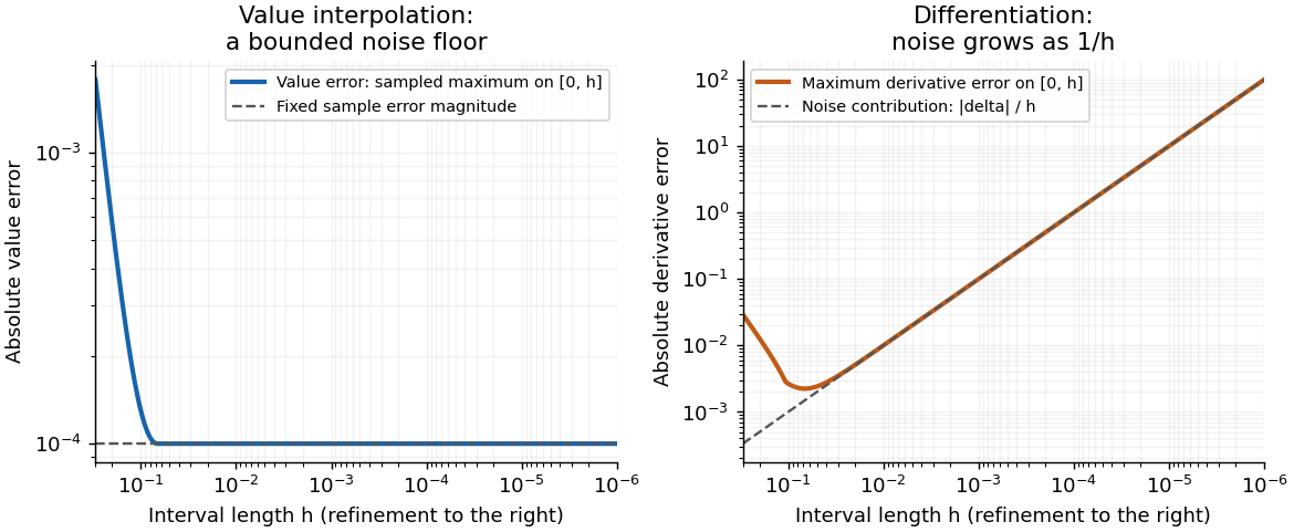
Write ${\tilde{p}}_1$ and $\tilde{q}$ for the quantities computed from the perturbed second sample. The endpoint linear interpolation and its derivative areCompare them on their interpolation interval $0\le x\le h$, with fixed $a>0$. Put $x=th$, $0\le t\le 1$. The Taylor series of the sine gives, uniformly in $t$,Here the second equality compares with $f^{\prime }(0)=a$. More generally, the exact derivative is $f^{\prime }(th)=a\cos (ath)$ andThe input perturbation itself changes the value interpolant by exactly $aϵx/h$, and changes its derivative by exactly $aϵ/h$. ThusFor fixed nonzero $ϵ$, the value approximation has a bounded noise floor: its maximum error approaches $a|ϵ|$, and at $x=h$ that error is exactly $a|ϵ|$. It does not converge uniformly to the exact values as $h\to 0$. However, it does not amplify the absolute sample perturbation on $[0,h]$. The derivative error instead grows without bound like $a|ϵ|/h$.

With exact samples, $ϵ=0$, both approximations do converge on the shrinking interval: the value error is $O(h^3)$ for this particular sine, and the derivative error is $O(h^2)$. With step-dependent noise, value convergence requires $ϵ(h)\to 0$, whereas derivative convergence requires the stronger $ϵ(h)=o(h)$, where $o$ denotes little o notation.

This is noise amplification by differentiation of a linear interpolant. Value interpolation has an absolute perturbation bound independent of $h$ on the sampled interval. Numerical differentiation has a perturbation factor $1/h$, expressing the ill-posedness of numerical differentiation from values with fixed absolute uncertainty. The amplification follows from the mathematical data map even in exact arithmetic; it is distinct from additional roundoff error in a particular implementation. For fixed $x$ outside $[0,h]$, the operation becomes extrapolation, and the value perturbation $aϵx/h$ can also diverge.

With zero boundary values eliminated, the diagonal of $L_h$ is $-4I/h^2$. The Jacobi method is thereforewhich averages the four neighboring components. The sine addition identity shows that the supplied product vectors are eigenvectors, withThe discrete sine vectors form a basis, so these are all eigenvalues. Their largest modulus isattained at the lowest and highest sine frequencies. Thus the asymptotic error reduction factor per iteration is $\cos (\pi h)$. If the convergence rate is expressed logarithmically, $R=-\log \rho (J)\sim {\pi }^2{h}^2/2$ as $h\to 0$. A fixed error reduction therefore takes $O(h^{-2})$ Jacobi sweeps. For the special grid $m=2$, $J=0$ and one sweep solves its single interior equation.

The endpoint $\alpha =0$ in the printed nonnegative-parameter hypothesis must be excluded. We first establish the intended result for $\alpha >0$, then describe that endpoint exactly.

Write $X,Y$ for the two directional matrices; they commute because they act on separate tensor-product coordinates. At a limit $V$, the intermediate vector also has a limit $\tilde{V}$. Subtract the two limiting equations in the form that cancels $X\tilde{V}$ and $YV$; this gives $2\alpha (\tilde{V}-V)=0$. Hence $\tilde{V}=V$ for $\alpha >0$. Substitution then gives $(X+Y)V=h^{2}f$, precisely the required discrete equation.

Eliminating the intermediate vector gives the alternating direction implicit iteration matrixThe sine-product basis simultaneously diagonalizes $X,Y$, with eigenvalues $-{\xi }_p$ and $-{\eta }_q$, whereThusFor $\alpha >0$, each factor has modulus strictly less than one. Hence $\rho (G)<1$, proving convergence from every starting vector to the unique discrete solution.

At $\alpha =0$ the two factors are both $-1$, so $G=I$. The forcing terms cancel in the composed iteration as well, and $V^{k+1}=V^k$ for every starting vector. An incorrect initial vector therefore remains incorrect forever, even though the sequence is constant and has a limit. This disproves both the literal fixed-point implication and the claimed general convergence-to-solution assertion at zero; strict positivity of $\alpha$ is the necessary repair.

For $u^{(m,n)}(x,y)=\sin (m\pi x)\sin (n\pi y)$, direct differentiation yieldsSince the planar Laplacian is $\Delta ={\partial }_{xx}+{\partial }_{yy}$, the required eigenvalue of $-\Delta +I$ isOn the sides $x=0,1$ the first sine factor vanishes, and on $y=0,1$ the second sine factor vanishes. Thus the homogeneous Dirichlet boundary condition holds on the whole boundary. The eigenfunction is nonzero, for instance at $(x,y)=(1/(2m),1/(2n))$, where its value is one.

The five-point Laplacian on the square grid isIt adds the second-order central differences in the two coordinate directions and uses the given zero Dirichlet boundary conditions when a neighbouring node lies on the boundary.

The sine addition formula impliesApply this identity with $\alpha =m\pi h$ in the $x$ direction and with $\alpha =n\pi h$ in the $y$ direction. For $U_{i,j}^{(m,n)}=\sin (m\pi ih)\sin (n\pi jh)$, it givesHence the discrete eigenvalues areBoth sine factors vanish on their respective boundary sides. Also $U_{1,1}^{(m,n)}>0$, since $m\pi /N$ and $n\pi /N$ lie strictly between zero and $\pi$. Thus each array is a nonzero discrete eigenvector, rather than merely the zero solution of the homogeneous system. The separated structure is also described by the five-point Dirichlet Laplacian as a Kronecker sum.

A fixed small-angle approximation alone is insufficient because its error is multiplied by $x$. Introduce the shrinking cutoff $\eta =x^{-1/3}$, which satisfies $\eta \ll ϵ$ but $\sqrt{x}\eta \to \infty$.

On $[0,\eta ]$, the Taylor expansion ${\sin }^{2}t=t^2+O(t^4)$ gives $x({\sin }^{2}t-t^2)=O(x{\eta }^4)=O(x^{-1/3})$ uniformly. Thusuniformly there, and the two central integrals are asymptotically equal. On $[\eta ,ϵ]$, choose a fixed $c>0$ with $\sin t\ge ct$ for $0\le t\le ϵ$. The sine-integral tail is at most $ϵe^{-c^{2}x{\eta }^2}=ϵe^{-c^2{x}^{1/3}}$; the Gaussian tail has the same exponential bound with $c=1$. Both are $o(x^{-1/2})$, while the central Gaussian integral is asymptotic to $\sqrt{\pi }/(2\sqrt{x})$. HenceThis justifies the localized Laplace method rather than interchanging a nonuniform approximation with integration.

Solving the time-independent Schrödinger equation with $\psi \propto e^{ik\varphi }$ gives $E={\hslash }^2{k}^2/(2m{R}^2)$. The periodic boundary condition requires $e^{2\pi ik}=1$, hence $k=n\in \mathbb{Z}$. With the angular integration measure $d\varphi$, wavefunction normalization givesso a convenient orthonormal eigenbasis isThe $n=0$ ground state is nondegenerate. For each $|n|>0$, $u_n$ and $u_{-n}$ span a two-dimensional energy eigenspace; real sine and cosine combinations are an equally valid basis. These opposite-circulation eigenstates have angular momentum $n\hslash$ and $-n\hslash$.

If instead the wavefunction is normalized with respect to physical arc length $ds=Rd\varphi$, its expression is $e^{in\varphi }/\sqrt{2\pi R}$. The two conventions describe the same probability, since $|u_n{|}^{2}d\varphi =|u_n/\sqrt{R}{|}^{2}ds$. The remaining parts use $d\varphi$.

A Fourier series separates a periodic physical signal into harmonics. For example, a periodic voltage applied to a linear circuit can be treated one frequency at a time; the harmonic responses then superpose to give the output waveform.

Write $w=\Delta T$ for the pulse width and $\delta =w/T$ for its duty cycle, with $0<w<T$. The waveform is a train of positive rectangular pulses centred on $t=jT$, each with area one. It is even about $t=0$, so every sine coefficient vanishes. Cosine orthogonality givesand, for $n\ge 1$,This is the Fourier series of a periodic rectangular pulse:The actual constant term in the series is $a_0/2=1/T$, not $a_0$. As usual for a jump discontinuity, the series converges to the average of the one-sided values at each pulse edge, namely $1/(2w)$, irrespective of the value assigned at that isolated endpoint. Elsewhere it converges to the rectangular waveform.

Counting the constant as the first term, the first three terms areso their sum isIf “first three” instead means the first three nonconstant harmonics, add $a_3\cos (6\pi t/T)$; the original plot shows that alternative partial sum as well. The three-term approximation rounds the narrow peaks and ripples between them; many harmonics are needed to represent a sharp pulse.

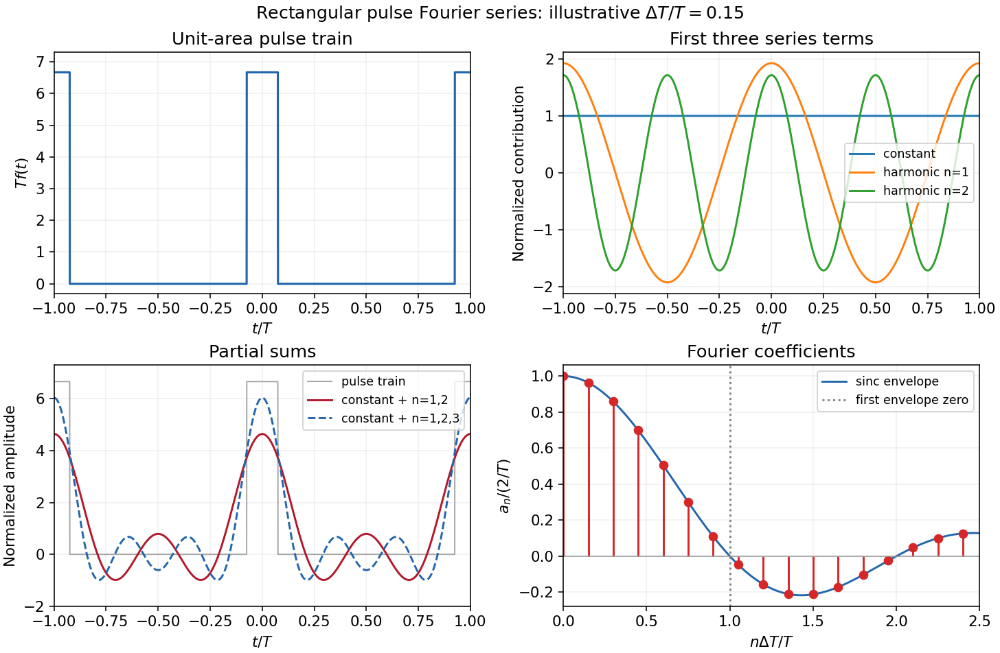
The original sketches use the illustrative duty cycle $\delta =0.15$ and cover $-T\le t\le T$. The coefficient panel also displays the first spectral zero.

For $n\delta \ll 1$, expand the sinc function:Thus the low-index coefficients, including $a_0$, have nearly equal values, although their constant-series contribution still has the factor $1/2$. The first sinc zero occurs at $n\delta =1$, or $n=T/w$. If this is not an integer, the closest integer coefficient is near zero rather than exactly zero: writing $n\delta =1+\epsilon$ gives $a_n\simeq -(2/T)\epsilon$. This pulse-width scale of Fourier coefficients means that a narrower pulse requires significant harmonics extending to proportionally larger indices, the reciprocal time-width/frequency-width relation.